Lecture 15: Linear Models with Normal Noise

Linear Gaussian model setup

In the previous lecture, we went through examples of inference involving some of the variations of Bayes' ruleBayes' rule Bayes' rule is the probability formula used to update beliefs about an unknown quantity after observing data.. One case that we did not consider was the case where the unknown random variablerandom variable A random variable is a numerical quantity whose value is determined by chance. and the observation are both continuous. In this lecture, we will focus exclusively on an important model of this kind. Because we consider only one specific setting, we will be able to study it in considerable detail.

Show notesHide notes

In the model that we consider, we start with some basic independentindependence / independence assumptions Independence means that random variables do not influence each other's distributions. normalnormal distribution / normal The normal distribution is a symmetric bell-shaped distribution described by a mean and a variance. random variablesrandom variable A random variable is a numerical quantity whose value is determined by chance.. Some of them, the theta_jTheta / thetas Theta is the unknown parameter or set of parameters being estimated in the model., are unknown, to be estimated. Some of them, the W_iW_i W_i is a noise term in the observation model., represent noise. Our observations, X_iXi / X1 up to Xn Xi is the i-th observation in a sequence of random variables., are linear functionslinear function / linear function of the measurements A linear function is a function formed from a linear combination of variables, often used to build simple estimators. of these basic random variables. In particular, since linear functions of independent normal random variablesnormal random variable A normal random variable has a normal distribution. are normal, the observations are themselves normal as well.

This is probably the most commonly used type of model in all of inference and statistics. This is because it is a reasonable approximation in many situations. Also, it has a very clean analytical structure and a very simple solution. For example, it turns out that the posterior distributionposterior distribution / posterior The posterior distribution is the distribution of a parameter after observing data and updating the prior with the likelihood. of each theta_jTheta / thetas Theta is the unknown parameter or set of parameters being estimated in the model. is itself normalnormal distribution / normal The normal distribution is a symmetric bell-shaped distribution described by a mean and a variance.. And the MAPMAP / MAP estimate MAP stands for maximum a posteriori estimate, the value of a parameter that maximizes its posterior distribution. and LMSLMS / least mean squares estimator LMS stands for least mean squares, an estimator defined here as the conditional expectation of Theta given the observation. estimates coincide. This is because the peak of a normal occurs at the mean.

Furthermore, these estimates are given by some simple linear functions of the observationslinear function / linear function of the measurements A linear function is a function formed from a linear combination of variables, often used to build simple estimators.. We will go over these facts by moving through a sequence of progressively more complex versions. We will start with just one unknown and one observation, and then generalize. And we will illustrate the formulation and the solution through a rather realistic example, where we estimate the trajectorytrajectory A trajectory is the path an object follows over time. of an object from a few noisy measurements.

Recognizing normal densities

In this lecture sequence, we will do a lot with normal random variablesnormal random variable A normal random variable has a normal distribution.. For this reason, it is useful to start with a simple observation that will allow us later on to move much faster. Recall that a normal random variable with a certain mean and variancevariance Variance measures the spread of a random variable or distribution around its mean. has a PDFPDF / probability distribution PDF stands for probability density function, the function used to describe a continuous probability distribution. of this particular form. What if somebody gives you a PDF of this form and asks you what it corresponds to? You can answer that this is exactly of this form, provided that you make the identification that 3 is equal to mu.

Show notesHide notes

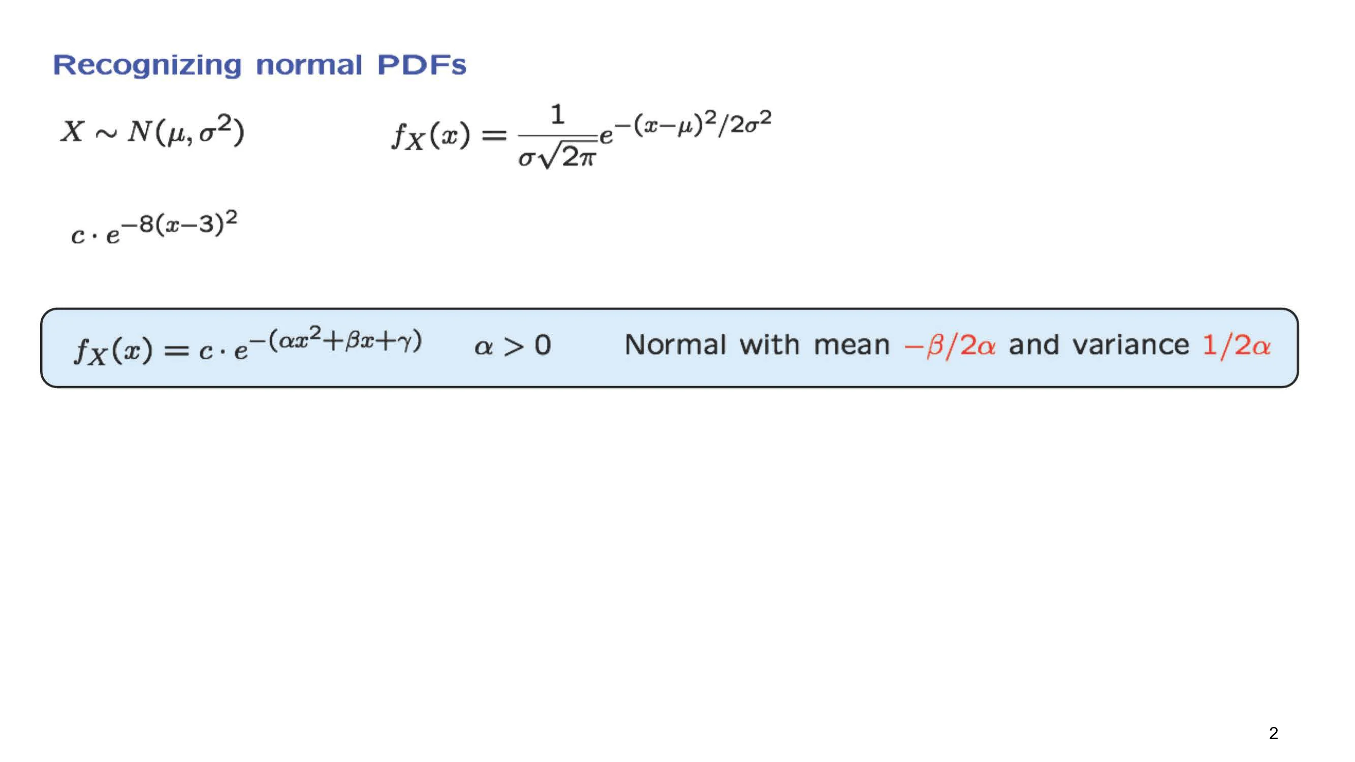
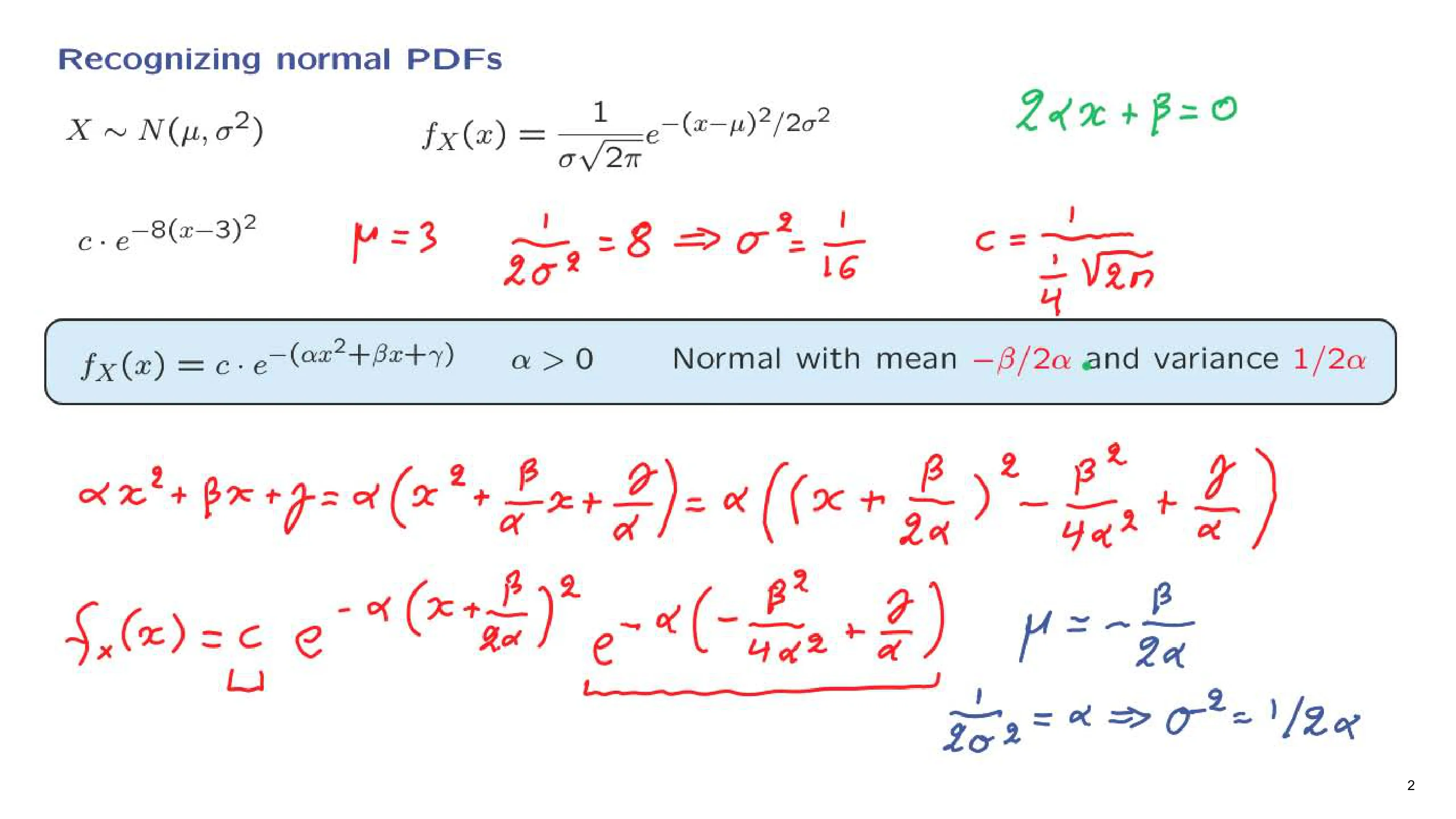
So this is a normal PDFPDF / probability distribution PDF stands for probability density function, the function used to describe a continuous probability distribution. with a mean equal to 3, and whose variancevariance Variance measures the spread of a random variable or distribution around its mean. can also be found by matching this constant that appears here with the number 8. This constant here is in the denominator, so we have a term 1 over 2 sigma squaredsigma squared Sigma squared is a notation for variance, especially in normal models.. This must be equal to 8. From this, we can infer that the variance of this random variable is equal to 1 over 16. If you also want to find out the value of this constant C, you check the formula for normal PDFnormal PDF A normal PDF is the probability density function of a normal distribution.s. The constant C is 1 over the standard deviation, which is 1/4 in our case, times the square root of 2 pi.

Now, suppose that somebody gives you a PDF of this form: a constant times the negative exponential of a quadratic functionquadratic function A quadratic function is a function with squared terms, such as a polynomial of degree two. in x. We will argue that this PDF is also a normal PDFnormal PDF A normal PDF is the probability density function of a normal distribution. and identify the parameters of that normal. First, let's start with a certain observation. A PDF must integrate to 1, so it cannot blow up as x goes to infinity, which means that this exponential needs to die out as x goes to infinity. That will only happen if this coefficient alpha here is positive, so that we have e to the minus something positive and large, which is going to die out. Therefore, alpha must be a positive constant, and let us assume from now on that this is the case.

What we will do next is try to write this PDF in this form. The trick that we're going to use is the following. We will focus on the term in the exponent, which we rewrite this way. We take out a factor of alpha, and then we will try to make this expression here appear like a square of this kind, like a perfect square. So what is involved is a certain method, a certain trick, called completing the squarecompleting the square Completing the square is an algebraic method for rewriting a quadratic expression in a more useful form..

That is, we write this term here in the form x plus something squared, and then we may need some additional terms. What should that something be? We would like that something to be such that when we expand this quadratic, we get this term and that term. We get an x squared, and then there's going to be a cross-term. What we need here so that the cross-term is equal to this is a term equal to beta over 2 alpha. Because in that case, the cross-term is going to be 2 times x times beta divided by 2 alpha. The 2 in the beginning and that 2 cancel out, so we're left with x beta over alpha, which is exactly what we got here.

However, this quadratic is going to have an additional term, which is going to be the square of this, which is not present here. So, to keep the two sides equal, we need to subtract that term. Finally, we have the last term involving gamma. Therefore, the PDF of x is of the form: we have a certain constant from here, then we have the negative exponential of this term, e to the minus alpha times the quantity x plus beta over 2 alpha squared. Then there's the negative exponential of the rest, which is going to be a term of the form e to the minus alpha times beta squared over 4 alpha squared plus gamma over alpha.

Now, this term here does not involve any x's, so it can be absorbed into the constant C. The dependence on x is only through this term. This term now looks exactly like what we've got up here, provided that you make the following identifications. Mu has to be equal to what we have here, but there's a minus sign here and no minus sign there, so mu is going to be the negative of what we have up here. It's minus beta over 2 alpha. As for sigma squaredsigma squared Sigma squared is a notation for variance, especially in normal models., we match and say that 1 over 2 sigma squared must be equal to the constant that we have up here, which is alpha. From this, we conclude that sigma squared is equal to 1 over 2 alpha.

So we have concluded that a PDF of this type is indeed a normal PDF. It has a mean equal to that value and a variance equal to that value. Actually, to figure out what the mean of this PDF is, we do not need to go through this whole exercise. Once we're convinced that this is a normal PDF, then we know that the mean is equal to the peak of the PDF. To find the peak, we want to maximize this over all x, which is the same as minimizing this quadratic functionquadratic function A quadratic function is a function with squared terms, such as a polynomial of degree two. over all x.

Where is this quadratic function minimized? To find that place, we can look at the exponent, take its derivative, and set it to 0. So setting the derivative of the exponent to 0 gives us the equation 2 alpha x plus beta equal to 0. From this, we solve for x, and we can tell that the peak of the distribution is going to be when x takes this particular value. This value must also be equal to the mean. So this is a very useful fact to know, and we will use it over and over: the negative exponential of a quadratic function of xnegative exponential of a quadratic function of x A negative exponential of a quadratic function is an expression like exp(−ax²−bx−c), which has the shape of a normal density. is always a normal PDF.

Single observation posterior

As a preparation for more complex and more difficult models, we will start by looking at the simplest model that involves a linear relationlinear relation A linear relation is a relationship between variables that can be written as a linear expression in the unknowns. and normal random variables. The specifics of the model are as follows. There is an unknown parameterunknown parameter An unknown parameter is a quantity in the model whose true value is not known in advance., modeled as a random variable, Theta, that we wish to estimate. What we have in our hands is Theta plus some additive noiseadditive noise Additive noise is random error or disturbance that enters a model by being added to the underlying quantity., W, and this sum is our observation, X.

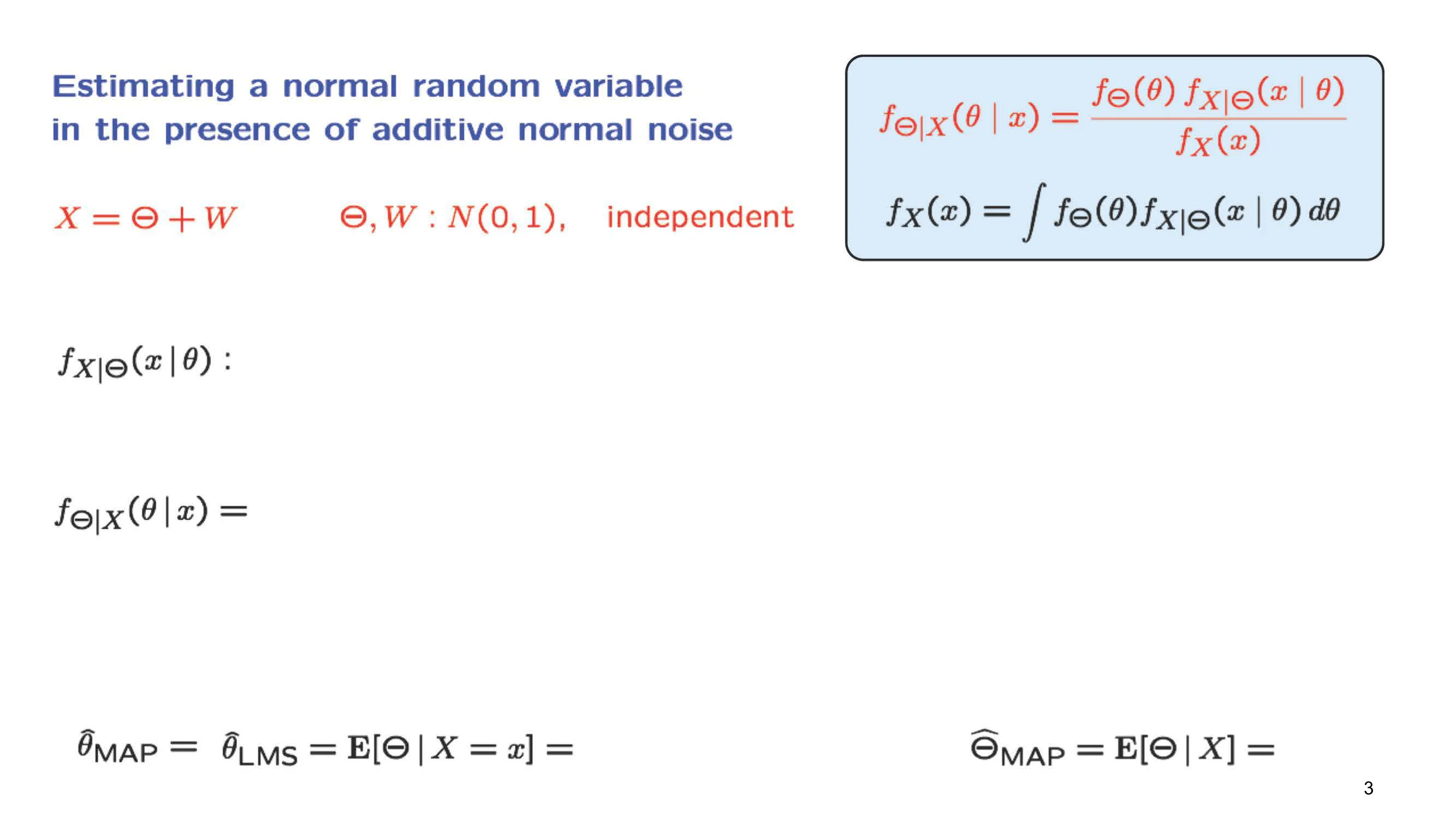
The assumptions that we make are that Theta and W are normal random variables. To keep the calculations simple, we assume that they are standard normal random variables. Furthermore, we assume that Theta and W are independentindependence / independence assumptions Independence means that random variables do not influence each other's distributions. of each other. According to the Bayesian program, inference about Theta is essentially the calculation of the posterior distribution of Thetaposterior distribution / posterior The posterior distribution is the distribution of a parameter after observing data and updating the prior with the likelihood. if I tell you that the observation, capital X, takes on a specific value, little x.

To calculate this posterior distribution, we invoke the appropriate form of Bayes' ruleBayes' rule Bayes' rule is the probability formula used to update beliefs about an unknown quantity after observing data.. We have the priorprior distribution / prior A prior distribution is the distribution assigned to a parameter before the data are observed. of Theta; it is a standard normal. Now we need to figure out the conditional distribution of X given Thetaconditional density / conditional density of X Conditional density is the density of a random variable given the value of another variable.. If I tell you that the random variable capital Theta takes on a specific value, little theta, then in that conditional universe our observation is going to be that specific value of Theta, which is little theta, plus the noise term, capital W.

Show notesHide notes

This is the relation that holds in the conditional universe where we are told the value of Theta. Now, W is independent of Theta, so even though I have told you the value of Theta, the distribution of W does not change. It is still a standard normal. So X is a standard normal plus a constant theta. What that does is change the mean of the normal distribution, but it will still be a normal random variable. In this conditional universe, X is going to be a normal random variable with mean equal to theta and with variance equal to the variance of W, which is equal to 1.

So now we know what this distribution is, and we can move on with the calculation of the posterior. We have the denominator term, which I am writing here, and then we have the density of Theta. Since it is a standard normal, it takes the form of a constant; we do not really care about the value of that constant. What we care about is the term in the exponent. Then we have the conditional density of X given Thetaconditional density / conditional density of X Conditional density is the density of a random variable given the value of another variable., which is normal with these parameters, and therefore takes the form C e to the minus one-half times X minus Theta, squared. This is the final form.

What we notice here is that we have a few constant terms, another term that depends on X, and then a quadratic in Theta. So we can write all this as some function of X and then e to the negative of some quadratic in Theta. When we are doing inference, we are given the value of X, so let us fix a particular value of little x and concentrate on the dependence on Theta. With X being fixed, this is just a constant, and as a function of Theta, it is e to the minus something quadratic in Theta. We recognize that this is a normal PDF, so we conclude that the posterior distribution of Theta, given our observation, is normal.

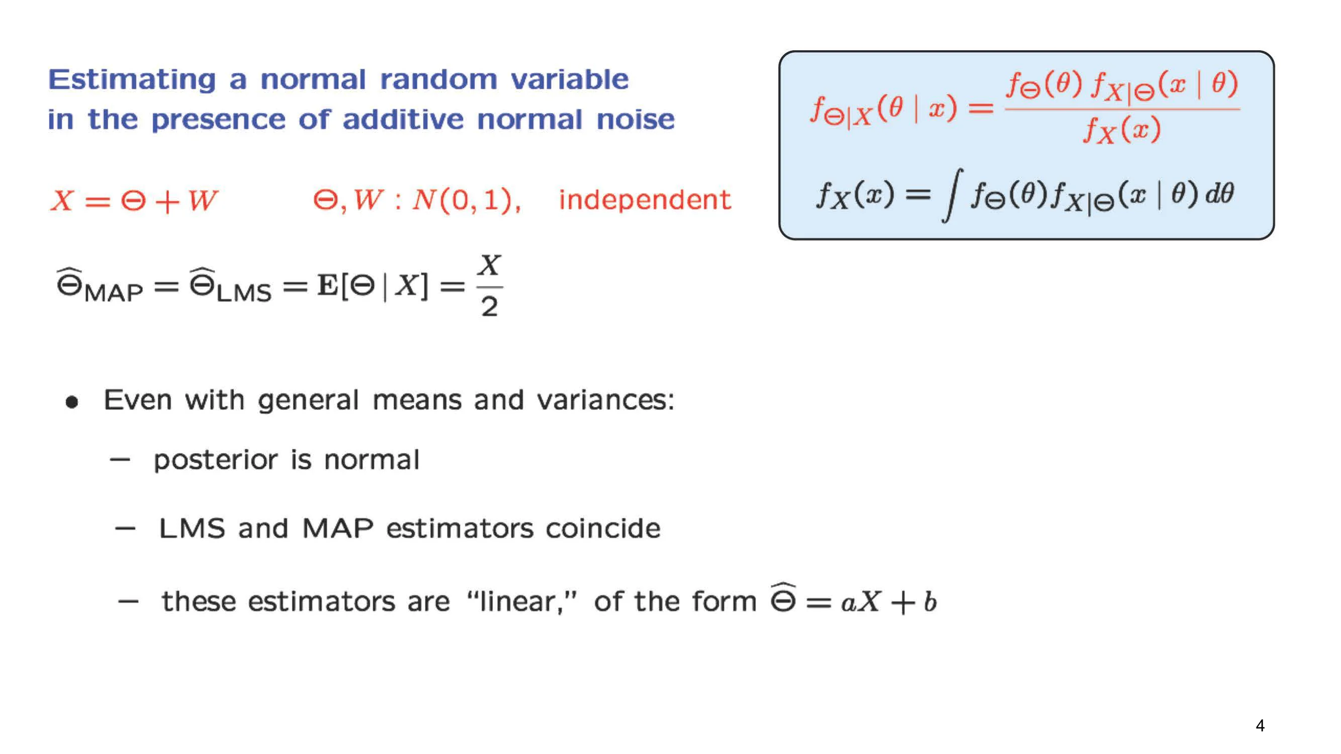
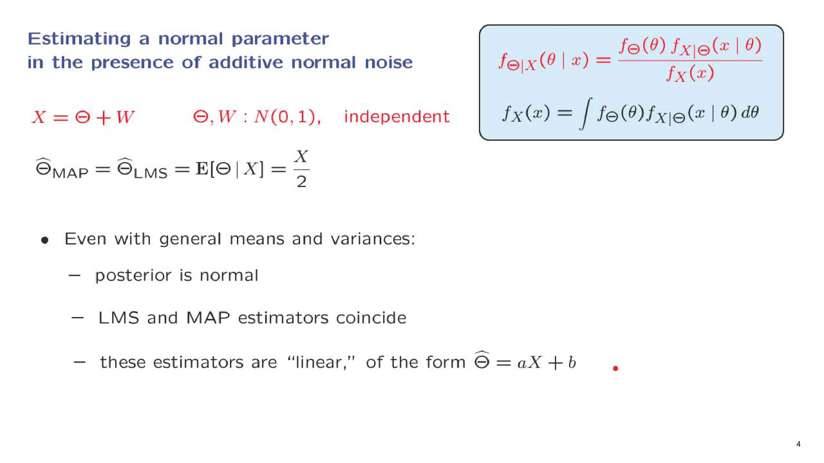
Since it is normal, the expected valueexpected value Expected value is the probability-weighted average of a random variable. of this conditional PDF will be the same as the peak of that PDF. This would be our point estimatepoint estimate A point estimate is a single value used to estimate an unknown parameter. of Theta, in particular if we use either the MAPMAP / MAP estimate MAP stands for maximum a posteriori estimate, the value of a parameter that maximizes its posterior distribution., maximum a posteriori probability, or the least mean squares estimatorLMS / least mean squares estimator LMS stands for least mean squares, an estimator defined here as the conditional expectation of Theta given the observation., which is defined as the conditional expectationconditional expectation Conditional expectation is the expected value of a random variable given another variable or observed data. of Theta given the observation that we have made. So this conditional expectation is just the mean of this posterior distribution. It is also the peak of that posterior distribution.

So let us find what the peak is. To find the peak, we focus on the exponent term, ignoring the minus sign. To find where the distribution peaks, we need to find the place where this exponent term is smallest. To find out when this term is smallest, we take its derivative with respect to Theta and set it equal to 0. The derivative of this term is Theta. The derivative of this term is Theta minus x. We set this to 0, and when we solve this equation, we find 2 Theta equal to x. Therefore, Theta is equal to x over 2.

So we conclude from here that the peak of the distribution occurs when Theta is equal to x over 2, and this is our estimate of Theta. Our estimate takes into account that we believe that Theta is 0 on the average, but also takes into account the observation that we have made and comes up with a value that is in between our priorprior distribution / prior A prior distribution is the distribution assigned to a parameter before the data are observed. mean, which was 0, and the observation, which is little x. So this is what the estimates are.

If we want to talk about estimatorestimator An estimator is a random-variable-valued rule that uses data to estimate an unknown parameter or signal.s, which are now random variables, what would they be? The estimator is a random variable that takes this value whenever capital X takes the value little x. Therefore, it is the random variable that is equal to capital X over 2. This is a relation between random variables. This is the corresponding relation between numbers if you are given a specific value for little x.

How special is this example? It turns out that the same structure of the solution shows up even if we assume that Theta and W are independent normal random variablesindependent normal random variables Independent normal random variables are Gaussian random variables that are independent of one another., but with some general means and variances. You should be able to verify on your own, by repeating the calculations that we just carried out, that the posterior distribution of Theta will still be normal. Since it is normal, the peak of the distribution is the same as the expected valueexpected value Expected value is the probability-weighted average of a random variable.. So the expected value, or least mean squares estimatorestimator An estimator is a random-variable-valued rule that uses data to estimate an unknown parameter or signal., coincides with the maximum a posteriori probability estimator.

Finally, although this formula will not be exactly true, there will be a similar formula for the estimators. Namely, the estimator will turn out to be a linear function of the measurements. We will see that these conclusions are actually even more general than that. This is what makes it very appealing to work with normal random variables and linear relationslinear relation A linear relation is a relationship between variables that can be written as a linear expression in the unknowns..

Multiple noisy measurements

We are now ready to move on to a model which is quite interesting and quite realistic. This is a model in which we have an unknown parameterunknown parameter An unknown parameter is a quantity in the model whose true value is not known in advance. modeled as a random variable that we try to estimate. This is the random variable Theta, and we have multiple observations of that random variable. Each one of those observations is equal to the unknown random variable plus some additive noiseadditive noise Additive noise is random error or disturbance that enters a model by being added to the underlying quantity..

Show notesHide notes

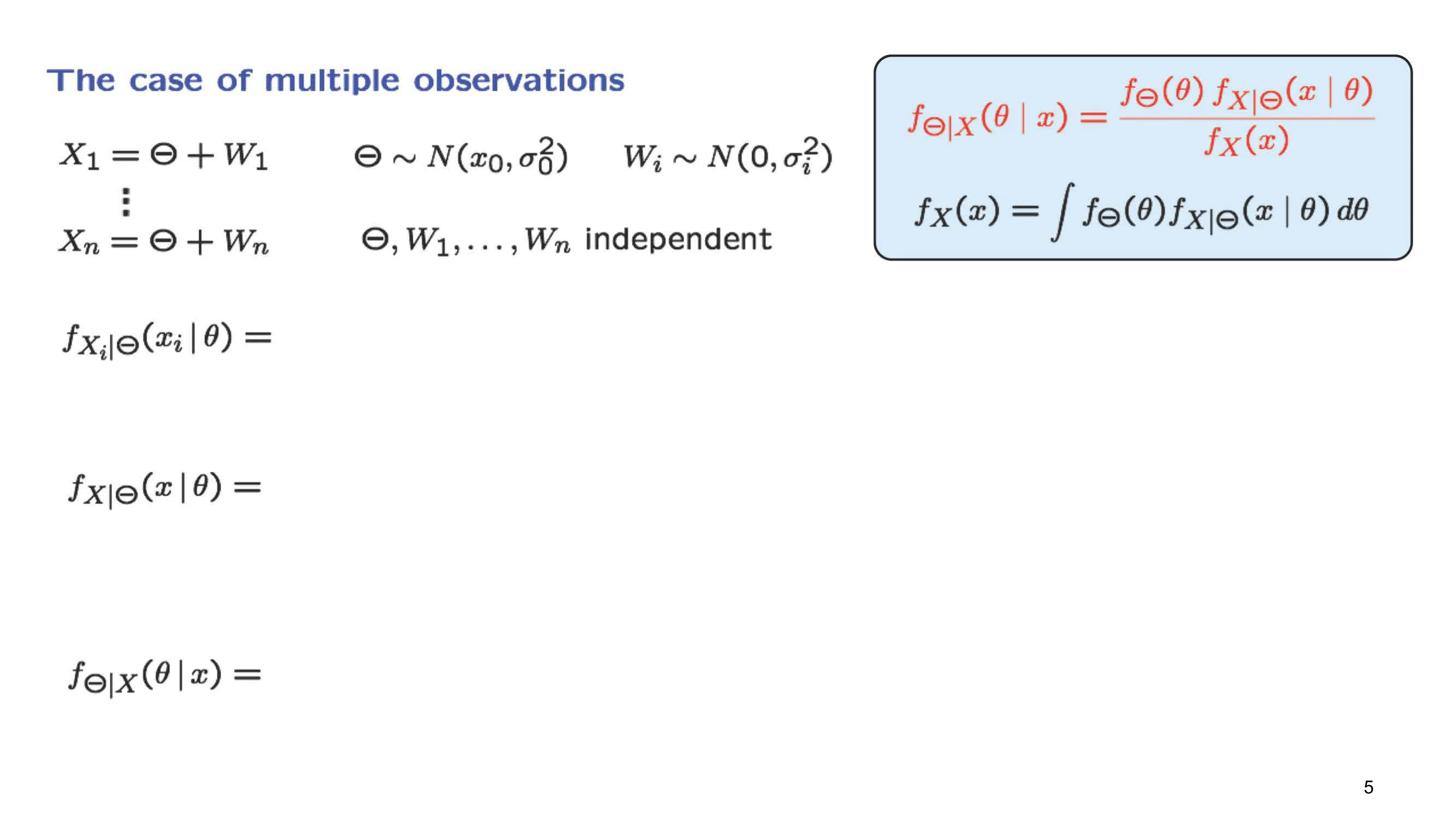
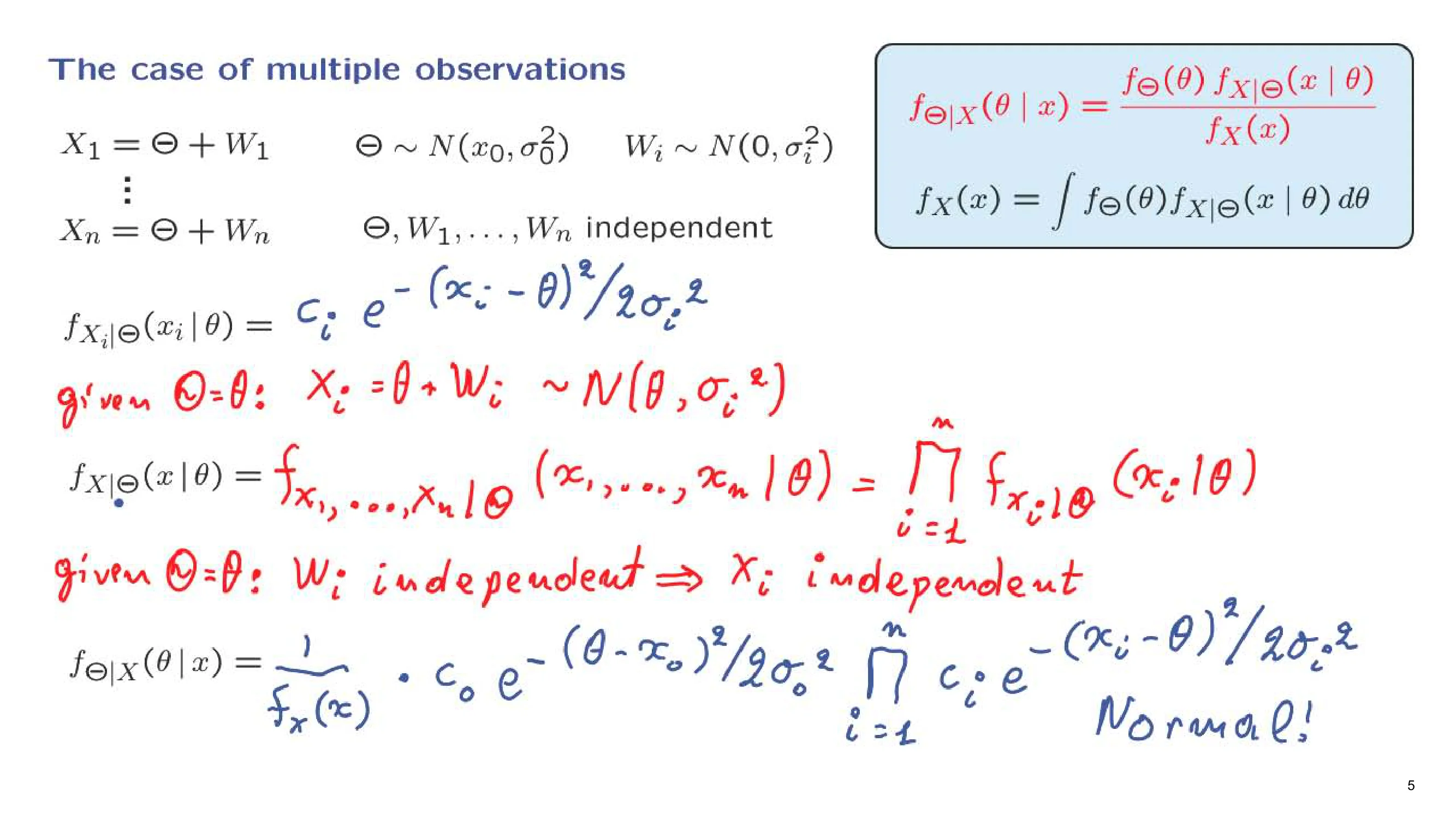
This is a model that appears quite often in practice. It is often the case that we're trying to estimate a certain quantity, but we can only observe values of that quantity in the presence of noise. Because of the noise, what we want to do is try to measure it multiple times. So we have multiple such measurement equations, and then we want to combine all of the observations together to come up with a good estimate of that parameter.

The assumptions that we will be making are that Theta is a normal random variable. It has a certain mean that we denote by x0x0 x0 is a model parameter used as the prior mean or initial value.; the reason for this strange notation will be seen later. It also has a certain variance. The noise terms are also normal random variables with 0 mean and a certain variance. Finally, we assume that these basic random variables that define our model are all independent.

Based on these assumptions, we would now like to estimate Theta on the basis of the X's. As usual, in the Bayesian setting, what we want to do is calculate the posterior distribution of Theta given the X's. Bayes' rule has the usual form for the case of continuous random variablescontinuous random variable / continuous random variables A continuous random variable is a random variable whose possible values form a continuum and are described by a density.. The only remark that needs to be made is that in this case there are multiple X's, so X here stands for the vector of the observations that we have obtained, and similarly little x stands for the vector of the values of these observations.

We need now to start making some progress toward calculating this term here: what is the distribution of the vector of measurements given Thetadistribution of the vector of measurements given Theta The distribution of the vector of measurements given Theta is the conditional distribution of the observed measurements for a fixed parameter value.? Before we move to the vector case, let us look at one of the measurements in isolation. This is something that we have already seen. If I tell you the value of the random variable Theta, which is what happens in this conditional universe when you condition on the value of Theta, then in that universe the random variable XiXi / X1 up to Xn Xi is the i-th observation in a sequence of random variables. is equal to the numerical value that you gave me for Theta plus WiW_i W_i is a noise term in the observation model..

Because Wi is independent from the random variable Theta, knowing the value of Theta does not change the distribution of Wi. It will still have this normal distribution. So Xi is a normal random variable of this kind plus a constant, and therefore Xi is a normal random variable with mean equal to the constant that we added and variance equal to the original variance of the random variable Wi. We can now write down the conditional PDF of Xi. There is going to be a normalizing constantnormalizing constant A normalizing constant is a factor that scales a function so it becomes a valid probability density., and then the usual exponential term, which is going to be Xi minus the mean of the distribution, which is Theta, divided by the usual variance term.

Let us move next to this distribution here. This is a shorthand notation for the joint PDFjoint PDF / joint density Joint PDF means joint probability density function, the density of several random variables taken together. of the random variables X1 up to Xn, conditional on the random variable Theta, so it is really a function of multiple variables. Here is the crucial observation: if I tell you the value of the random variable Theta as before, then all these random variables are independent. If I tell you the value of Theta, this does not change the joint distribution of the Wi's. The Wi's were independent when we started, so they remain independent in the conditional universe.

Since the Wi's are independent and the Xi's are obtained from the Wi's by just adding a constant, this means that the Xi's are also independent in this conditional universe. Once I tell you the value of Theta, then because the noises are independent, the observations are also independent. This means that the joint PDFjoint PDF / joint density Joint PDF means joint probability density function, the density of several random variables taken together. factors as a product of the individual marginal PDFsmarginal PDF / marginal density A marginal PDF is the probability density of one variable after the other variables in a joint distribution have been removed by integration. of the Xi's, and these PDFs we have already found.

So now we can put everything together to write down a formula for the posterior PDF using Bayes' rule. We have this denominator term, which I will write first, and which we do not need to evaluate. Then we have the marginal PDF of Thetamarginal PDF / marginal density A marginal PDF is the probability density of one variable after the other variables in a joint distribution have been removed by integration.. Since Theta is normal with these parameters, this is of the form e to the minus (Theta minus x0x0 x0 is a model parameter used as the prior mean or initial value.) squared over 2 sigma0 squared. Then we have this joint density of the X's conditioned on Theta, which we have already found. It is this product here, a product of n terms, one for each observation, and each one of these terms is what we found earlier.

Now, once we have obtained the observations, so the value of the random variable capital X, that is, the value little x, is fixed. Once it is fixed, the X's that appear here are constants. So in particular this term here is a constant, and we do not bother with it. What we have is a constant times an exponential in terms that are quadratic in Theta. So we recognize this kind of expression: it has to correspond to a normal distribution.

This is the first conclusion of this exercise: the posterior PDF of the parameter Theta, given our observations, is normal. We have e to a quadratic function in Theta, and that quadratic function also involves the specific values of the X's that we have obtained. Let us copy what we have found and rearrange it. Once more, we have a constant, then the exponential of the negative of some quadratic function in Theta, and the specific quadratic function that we calculated just before takes this particular form.

Show notesHide notes

Show notesHide notes

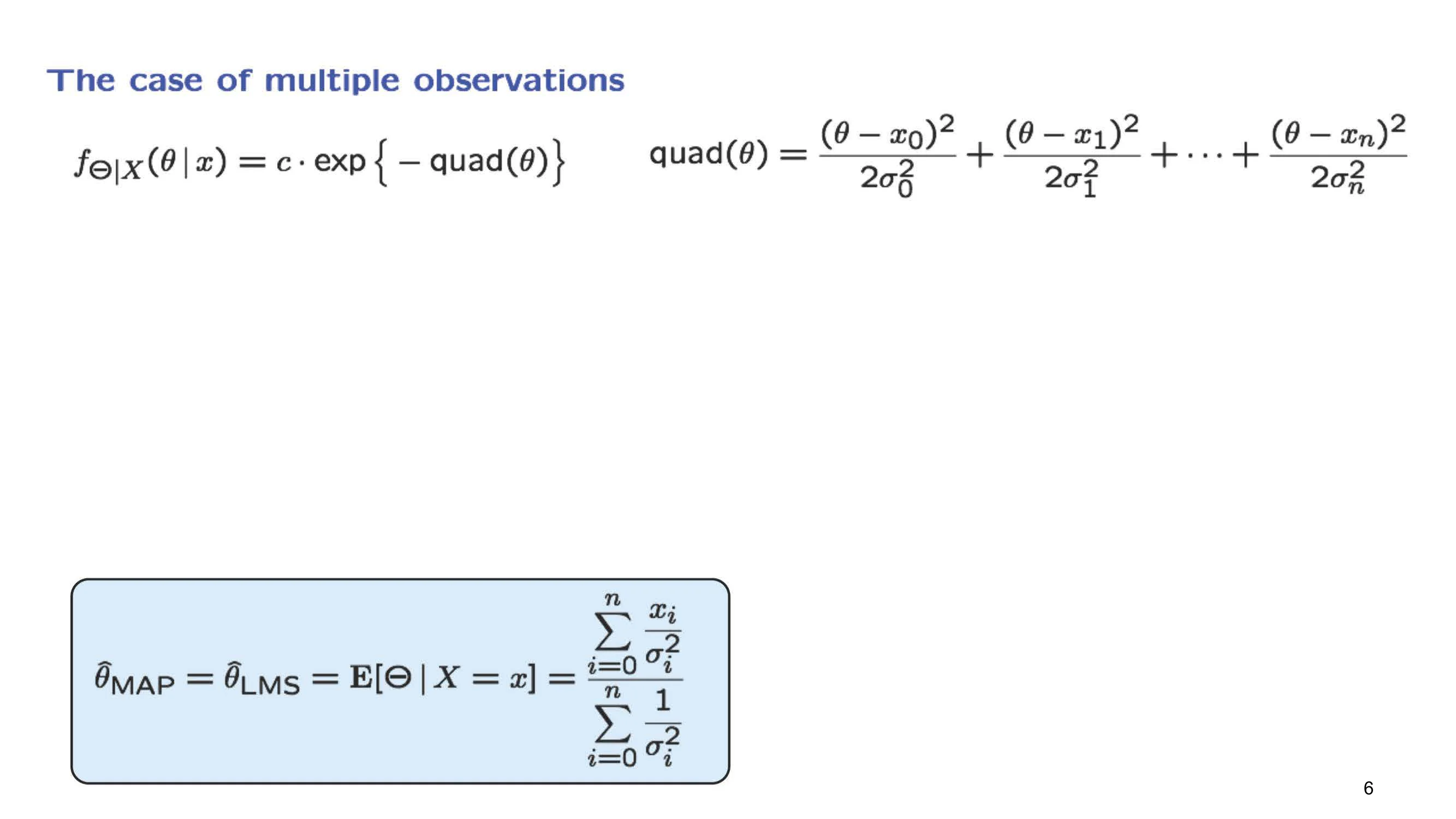
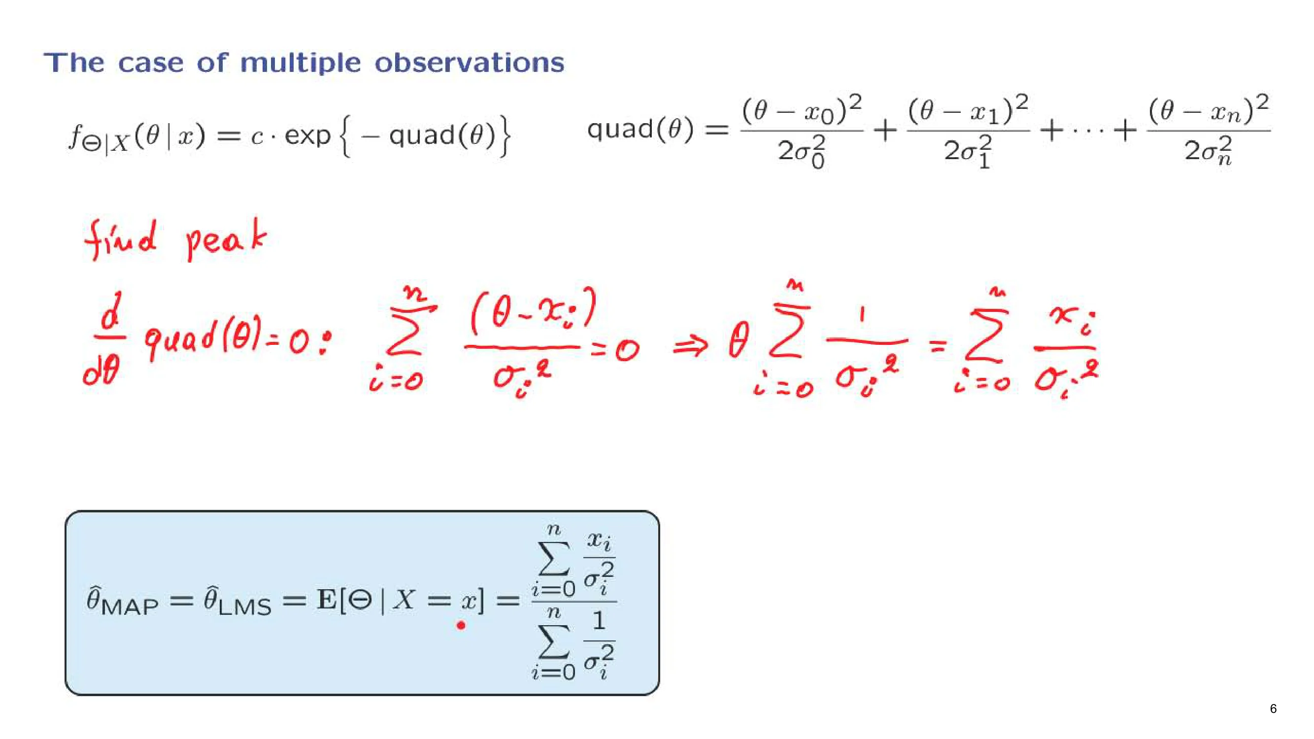
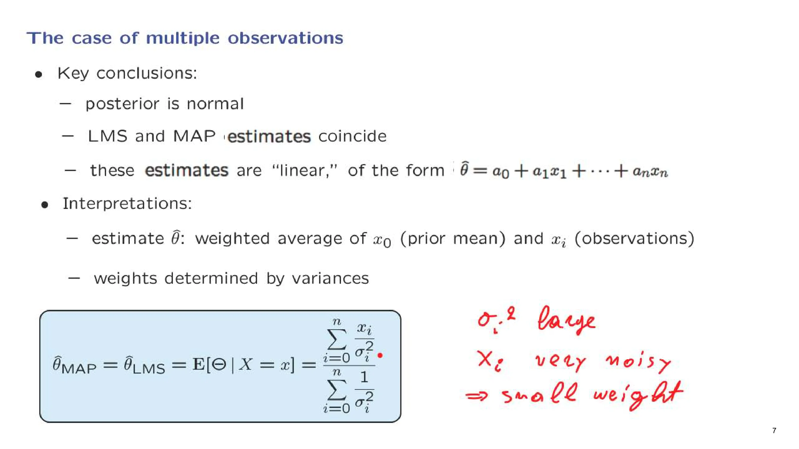
What is the mean of this normal distribution? The mean is the same as the peak. To find the peak, the location at which this PDF is largest, we try to find the place at which this quadratic function is smallest. So we take the derivative with respect to Theta of this quadratic and set it to 0. This gives us a sum of terms. The derivative of the typical term is going to be Theta minus Xi divided by sigma i squared, and this expression must be equal to 0 if Theta is at the peak of the posterior distribution.

We now rearrange this equation. We split off the term involving Theta, and this gives us a contribution of this kind. We move the terms involving the X's to the other side, and this gives us this expression. Finally, we take this sum here and send it to the denominator on the other side, and this gives us the final form of the solution. The peak of the posterior distribution is also the same as the conditional expectationconditional expectation Conditional expectation is the expected value of a random variable given another variable or observed data. of the posterior distribution. Whenever we have a normal distribution, the expected value is the same as the place where the distribution is largest.

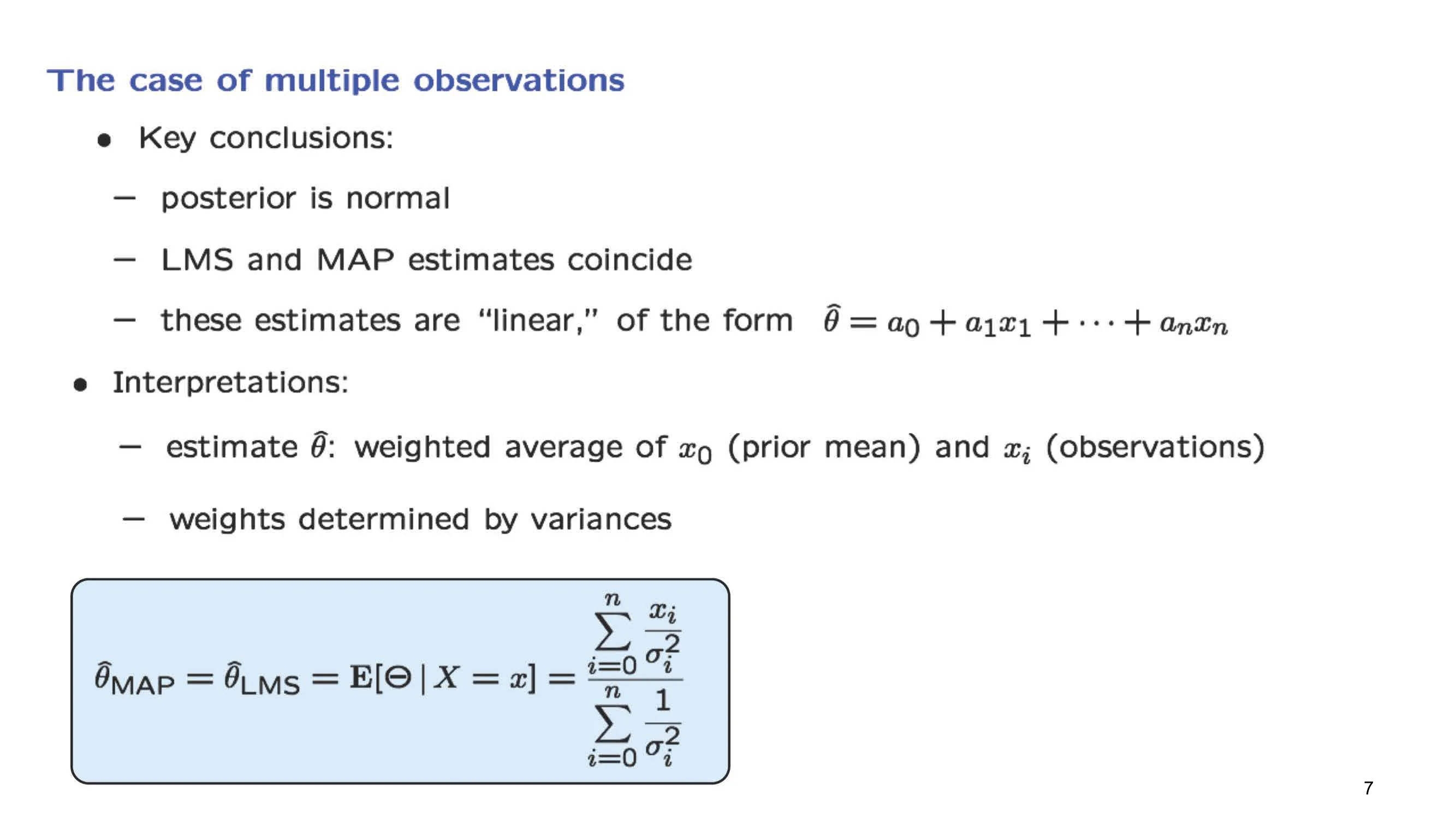
Let us now conclude with a few comments about how to interpret the result that we found. First, let me emphasize that the same conclusions that we obtained for the case of a single observation go through in this case as well. The posterior distribution of the unknown parameter is still a normal distribution. Our state of knowledge about Theta after we obtain the observations is described by a normal distribution. Because it is a normal distribution, the location of its peak is the same as the expected value.

For this reason, the conditional expectation estimate and the maximum a posteriori estimate coincide. Finally, the form of the estimate that we get is a linear function of the Xi's. This linearity is a very convenient property to have, because it allows further analysis of these ways of obtaining estimates. How do we interpret this formula? What we have here is the following: each one of the Xi's gets multiplied by a certain coefficient, which is 1 over the variance. And in the denominator, we have the sum of all those coefficients. So what we really have here is a weighted averageweighted average A weighted average is an average where some values count more than others. of the Xi's. Keep in mind that those Xi's are not all of the same kind. One term is X0, which is the prior meanprior mean The prior mean is the expected value of a parameter before data are observed., whereas the remaining Xi's are the values of the observations.

So there's something interesting happening here. We combine the values of the observations with the value of the prior meanprior mean The prior mean is the expected value of a parameter before data are observed.. In some sense, the prior mean is treated as just one more piece of information available to us, and it is treated in a sort of equal way as the other observations.

The weights that we have in this weighted averageweighted average A weighted average is an average where some values count more than others. are such that each Xi gets divided by the corresponding variance. Does this make sense? Suppose that sigma i squared is large. This means that the noise term Winoise term Wi Wi is the noise term for the i-th observation in the model. is very large, so Xi is very noisy. And so it's not a useful observation to have. In that case, it gets a small weight.

So the weights are determined by the variances in a way that is quite sensible. Those observations that will get the most weight will be those observations for which the corresponding noise variancenoise variance Noise variance is the variance of the random error terms in a model. is small. So the solution to this estimation problemestimation problem An estimation problem is a statistical problem in which the goal is to infer an unknown quantity from observed data. that we just went through has many nice properties.

First, we stay within the world of normal random variables, because even the posterior is normal. We stay within the world of linear functions of normal random variableslinear functions of normal random variables Linear functions of normal random variables are weighted sums or affine combinations of Gaussian variables.. And the form of the formula that we have itself has an appealing intuitive content.

Posterior variance and error

We now continue our discussion of the model in which we obtain several measurements of an unknown random variable Theta in the presence of additive noise, under the same assumptions as before. Theta and Wi are all independent random variables, and they are also normal. We have seen that in this case, the posterior distribution of Theta is a normal distribution and takes this particular form. We found the mean of the posterior distribution, which is also the maximum a posteriori probability estimate, and it is given by this expression.

Show notesHide notes

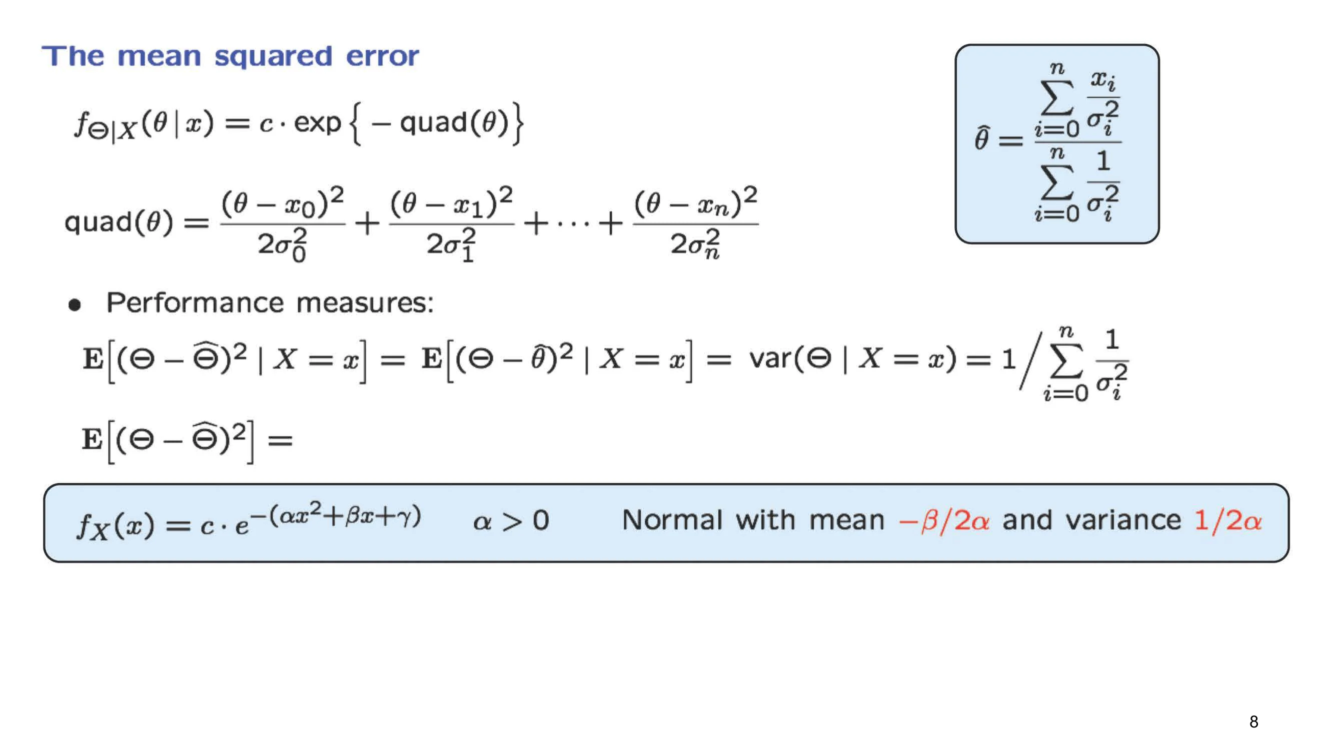
Now that we have an estimate in our hands, we can ask how good this estimate is. For this, we need an appropriate performance measure. For estimation problemestimation problem An estimation problem is a statistical problem in which the goal is to infer an unknown quantity from observed data.s, a reasonable performance measure is to look at the mean value of the squared error. But given that we have already obtained observations, what we are interested in is the conditional mean squared errorconditional mean squared error Conditional mean squared error is the mean squared error of an estimator given the observed data or another conditioning variable.. This is the error that is remaining after we have seen the observations.

Now, let us notice something here. If I tell you the value of the observations, then my estimator is completely determined. The estimator is a random variable that processes the data and comes up with an estimate. So although it is a random variable, once I tell you the value of the observations, the value of this random variable has been completely determined. And so we can replace it with its actual numerical value, which is Theta hatTheta hat Theta hat is the estimate of Theta obtained from the data., and it is given by this expression.

Now, remember also that Theta hatTheta hat Theta hat is the estimate of Theta obtained from the data., the estimate that we are using, is the mean of the posterior distribution. In this conditional universe, where we have conditioned on this information, Theta hat is the mean of this random variable. So we are dealing with the squared distance from the mean, and then we take the expected value. But that is nothing but the variance of Theta in this conditional universe. So what we are looking for is the variance of the posterior distribution of Theta, given the observations that we have obtained.

Can we eyeball the variance by just looking at this formula for the posterior distribution? More or less, we can. Recall this earlier fact, that if I give you a density of this form, you recognize that it is normal, and you also recognize that the variance is determined by the coefficient that comes next to the term of the form x squared. Now, this is a PDF involving a variable x. Here, we are talking about a PDF of Theta. So what we are looking for is the constant that sits next to the Theta squared term.

There are going to be multiple Theta squared terms, so we need to collect all of them. And so we find that the overall coefficient sitting next to the Theta squared terms is as follows. From this, we obtain a contribution of 1 over 2 sigma 0 squared. And similarly, from here, we are going to obtain a coefficient next to Theta squared of 1 over 2 sigma 1 squared. We continue the same way. And finally, from the last term, we obtain a contribution of this kind.

Now, we take this factor of 2, move it to the other side, so we know what 2 times alpha is. And then we need to take the inverse of that, so as to obtain 1 over 2 alpha. And what we obtain is that 1 over 2 alpha, when alpha is given by this expression, is equal to this expression here. And so we have found the conditional varianceconditional variance Conditional variance is the variance of a random variable given another variable or observed data., the variance of the posterior distribution of Theta, given the data that we have available in our hands.

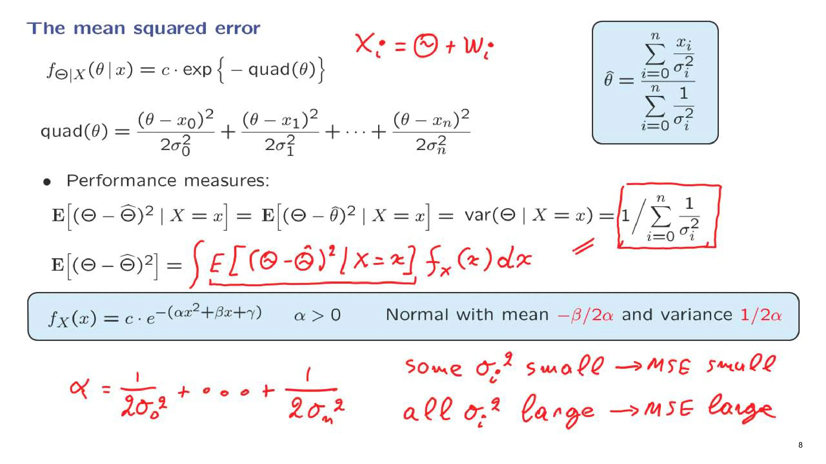
Now, this is the mean squared errormean squared error Mean squared error is the average squared difference between an estimate and the true parameter value., given that you have seen some particular piece of information. What about the overall mean squared error? This is the quantity that you care about before you go and make the actual measurements. This tells you how well you expect to estimate your random variable Theta. We can use here the total expectation theoremtotal expectation theorem The total expectation theorem says that an expectation can be found by taking a conditional expectation and then averaging it. and write the expected value as a weighted average of the conditional expectations under different scenarios, namely under different measurements of x, and average those conditional expectations over the possible values of x.

Now, this quantity here is actually a constant. It is this constant here. So we can pull it outside the expectation. What we are left with is the integral of a PDF over all possible values, which has to be equal to 1. So what we are left with is just the value of this constant, which is this particular number. And so we conclude that the overall unconditional mean squared errormean squared error Mean squared error is the average squared difference between an estimate and the true parameter value. is also the same. This makes perfect intuitive sense. Our mean squared error is going to take this value no matter what I observe, so on the average it will also take that particular value.

Now, this expression that we have derived is also quite intuitive in its content. Let us try to understand some special cases. Suppose that one of the variances of the noise terms is very small. If one term is small, this means that the corresponding term here is going to be big. So the sum of those terms is going to be big. As long as one term is big, then the sum is also big. And then 1 over that is going to be small. So in that case, the mean squared error is small.

What this is saying is that if just one of the measurements has low noise, then the uncertainty that remains for my random variable that I am trying to estimate will be small. I am going to have a small error. On the other hand, if all of the noise variancesnoise variance Noise variance is the variance of the random error terms in a model. are large, then this means that all of these terms here are going to be small. I am adding small terms. One over something small is something big. And so the mean squared error is going to be large. That is, if all my measurements are very noisy, then I do not expect to estimate my random variable particularly well.

Show notesHide notes

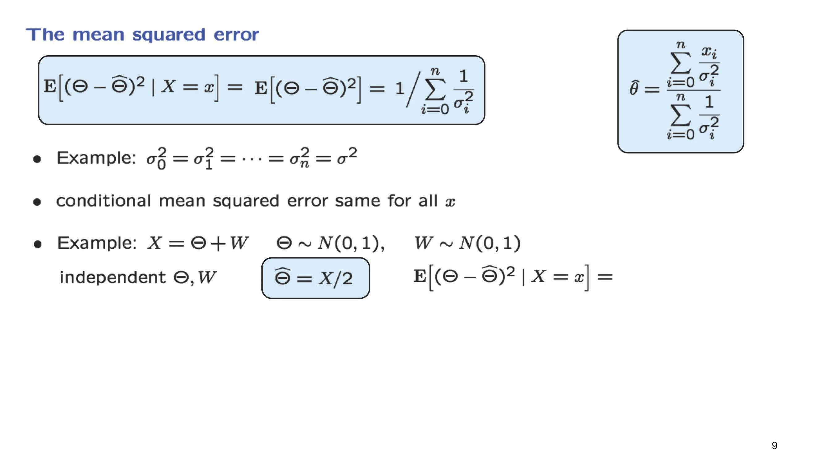
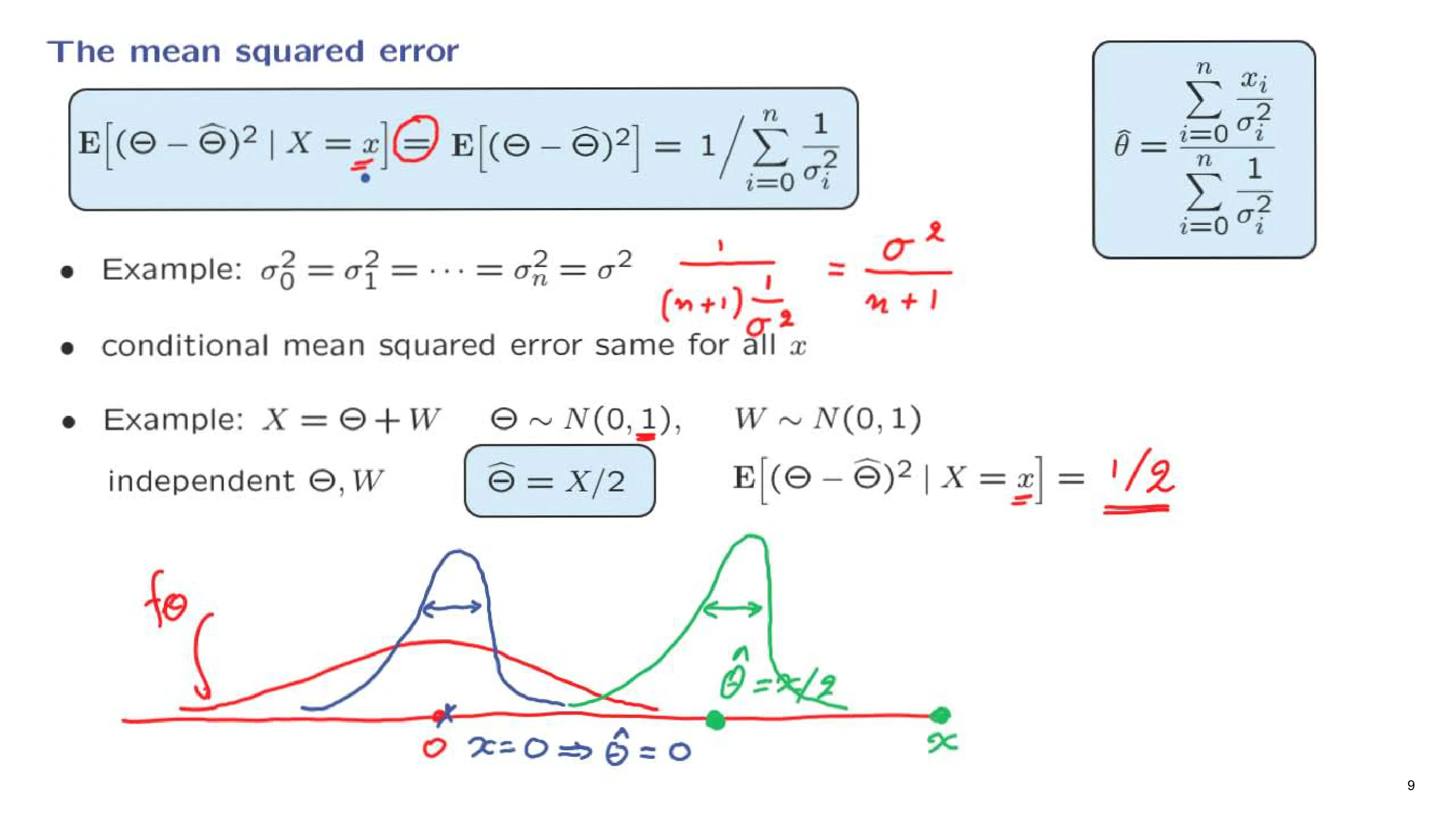
Let us now look at one more special case. Suppose that all the variances are the same, the noise variances as well as the variance of the prior distribution. In that case, this expression here is going to become 1 over the sum of n plus 1 terms, and each one of those terms is 1 over sigma squared, which is the same as sigma squared over n plus 1. This expression makes quite a lot of sense. It tells us that if we obtain more and more observations, that is, as n increases, we improve our performance. The variance of the posterior distribution, or the mean squared error, goes down in this particular way.

Now, perhaps the most interesting aspect of the facts that we have established is this equation here that tells us that no matter what this value of little x is, the conditional varianceconditional variance Conditional variance is the variance of a random variable given another variable or observed data., the variance of the posterior distribution of Theta, is going to be the same. In some sense, it tells us that no particular value of x is more informative or more desirable than any other value. In order to really appreciate what that statement is saying, it is better to look at a very concrete example.

So let us revisit the very first example that we studied, in which case we only have one observation, and where Theta and W are standard normal random variables. We did go through that example, and we found that the estimator, the maximum a posteriori probability estimator, was one-half of the observation. And now we are in a position to also calculate the conditional mean squared errorconditional mean squared error Conditional mean squared error is the mean squared error of an estimator given the observed data or another conditioning variable. given any particular observation. We apply this formula. In fact, we are dealing with this special case with sigma equal to 1. So we use this expression here, and we see that it is one-half.

So we started with a prior varianceprior variance The prior variance is the spread of a prior distribution before observing data. for Theta, which was 1, and after we obtained the observation, our uncertainty gets reduced, and the variance goes down to one-half. And this is true no matter what little x is. Pictorially, here is what is happening. We start with Theta being a standard normal, so it has a distribution of this form centered at 0. This is a plot of the density of Theta, the prior density. Suppose that we obtain a measurement, and that measurement happens to be equal to 0. If the measurement is equal to 0, then our estimate will also be equal to 0. The posterior distribution of Theta is going to be a normal distribution whose mean is the estimate and whose variance is this quantity that we have calculated, which is one-half. Therefore, it is narrower than the original PDF that we started from. Initially, we had a fair amount of uncertainty about Theta. After we obtain a measurement of 0, this reinforces our belief that Theta is somewhere near 0, and so we obtain a narrower distribution. This is our updated belief about Theta.

But what if I happen to obtain a measurement that's somewhere out here? In this case, my estimate is going to be one-half of what I observed. The posterior PDF of Theta is going to be a normal PDF that's centered around this point and has the same variance, one-half.

In some sense, this particular measurement would be thought of as quite an abnormal one. We're really surprised to obtain an observation that is so far away from 0, because our prior distribution told us that Theta is somewhere here. So we have been surprised. But after the surprise, and after we form our estimate of Theta, our state of knowledge about Theta is that Theta is a random variable, and it has a distribution that's normal, centered around this point, and whose width is the same no matter what particular observation I happen to get.

So even though this particular observation value is unusual, after it is obtained, the remaining uncertainty about Theta is the same as if we had obtained any other particular value of X. This is a very remarkable property that's special to this type of estimation problems involving normal random variables and linear relations. It has a very nice side effect. It means that we can say anything there is to be said about the performance of this maximum a posteriori probability estimator by just giving a single number. We can characterize performance only in terms of this number, as opposed to having to tell what this conditional mean squared error is for the different values of X.

Trajectory estimation model

In this segment, we introduce a model with multiple parameters and multiple observations. It is a model that appears in countless real-world applications. But instead of giving you a general and abstract model, we will talk about a specific context that has all the elements of the general model, with the advantage of being concrete, and we can also visualize the results.

Show notesHide notes

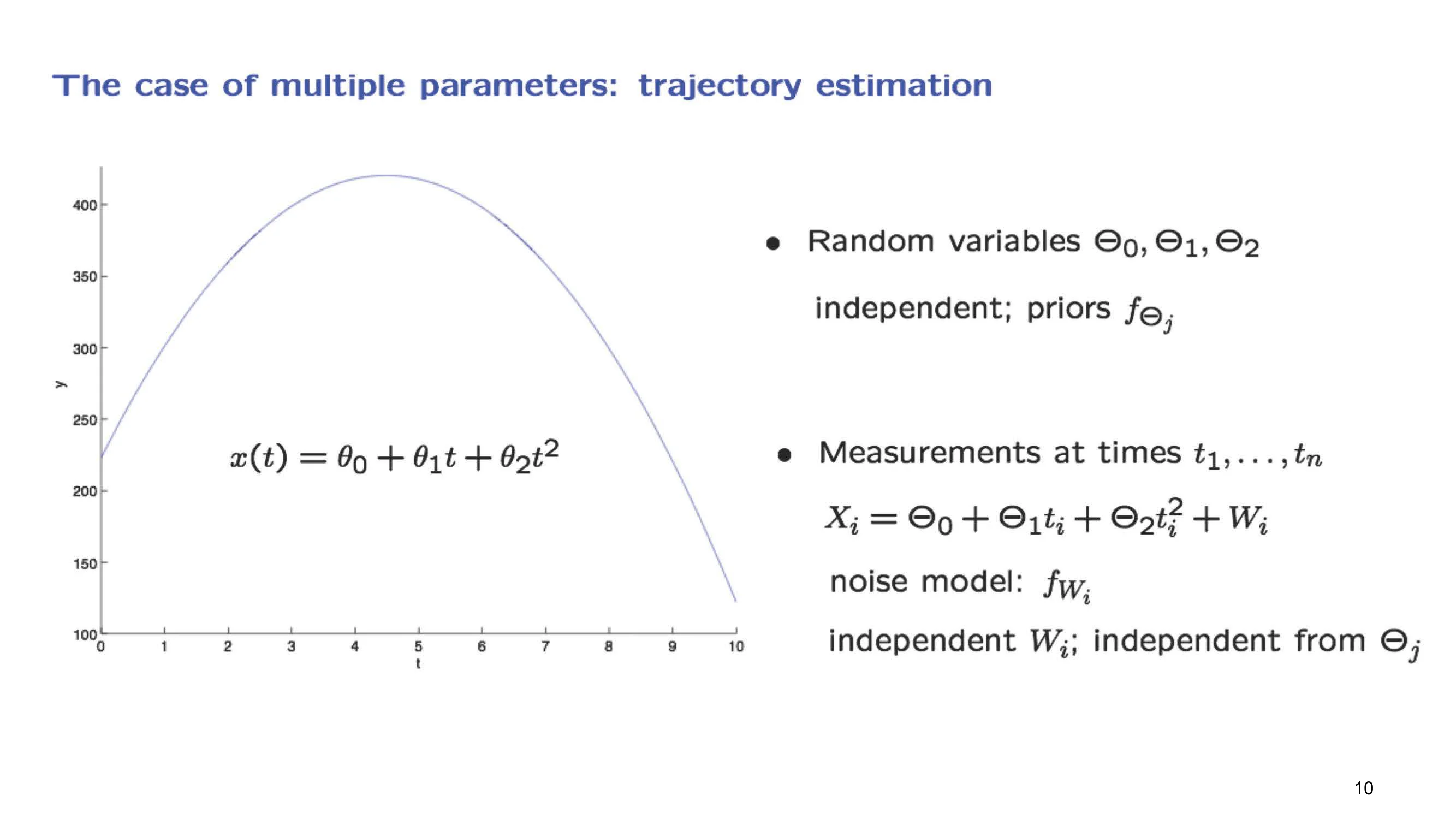
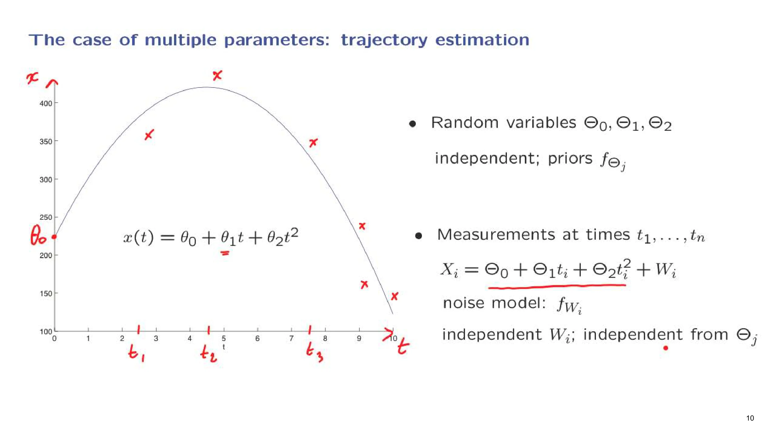
The model is as follows. Somebody is holding a ball and throws it upwards. This ball is going to follow a certain trajectorytrajectory A trajectory is the path an object follows over time.. According to Newton's laws, we know that it is going to be described by a quadratic function of time. Here, the time axis is horizontal, and the variable x is the vertical displacement of the ball. The ball initially is at a certain location, at a certain height, theta 0theta components / theta 0 Theta components are the separate parameters that make up the full Theta vector.. It is thrown upwards, and it starts moving with some initial velocity, theta 1. But because of the gravitational force, it will eventually start going down. So this parameter theta 2, which will actually be negative, reflects the gravitational constant.

Suppose now that you do not know these parameters. You do not know exactly where the ball was when it was thrown. You do not know the exact velocity. And perhaps you also live in a strange gravitational environment, and you do not know the gravitational constant. You would like to estimate those quantities based on measurements.

If you are to follow the Bayesian inference methodologyBayesian inference / Bayesian inference methodology Bayesian inference is a method for estimating unknown quantities by combining prior information with observed data., what you need to do is to model those variables as random variables, and think of the actual realized values as realizations of these random variables. We also need some prior distributions for these random variables. We should specify the joint PDF of these three random variables. A common assumption here is to assume that the random variables involved are independent of each other, and each one has a certain prior.

Where do these priors come from? If, for example, you know where the person is that's throwing the ball, if you know their location within, let us say, a meter or so, you should have a distribution for theta 0theta components / theta 0 Theta components are the separate parameters that make up the full Theta vector. that describes your state of knowledge, and which has a width, or standard deviation, of maybe a couple of meters. So the priors are chosen to reflect whatever you know about the possible values of these parameters.

Then what is going to happen is that you are going to observe the trajectory at certain points in time. For example, at a certain time, t1, you make a measurement, but your measurement is not exact. It is noisy, and you record a certain value. At another time, you make another measurement, and you record another value. At another time, you make another measurement, and you record another value. Similarly, you get multiple measurements. On the basis of these measurements, you would like to estimate the parameters.

Let us write down a model for these measurements. We assume that the measurement is equal to the true position of the ball at the time of the measurement, which is this quantity, plus some noise. And we introduce a model for these noise random variablesnoise random variables Noise random variables are the random terms in a model that represent disturbance, error, or unexplained variation.. We assume that we have a probability distribution for them. We also assume that they are independent of each other and independent from the thetas.

It is quite often the case that measuring devices, when they try to measure something multiple times, produce noises that are independent. So this is often a realistic assumption. In addition, the noise in the measuring devices is usually independent from whatever randomness there is that determined the values of the phenomenon that you are trying to measure. So these are pretty common and realistic assumptions.

Let us take stock of what we have. We have observations that are determined according to this relation, where Wi are noise terms. Now let us make some more concrete assumptions. We will assume that the random variables, the thetas, are normal random variables. Similarly, the W's are normal. As we said before, they are all independent. And to keep the formulas simple, we will assume that the means of those random variables are 0, although the same procedure can be followed if the means are nonzero.

Show notesHide notes

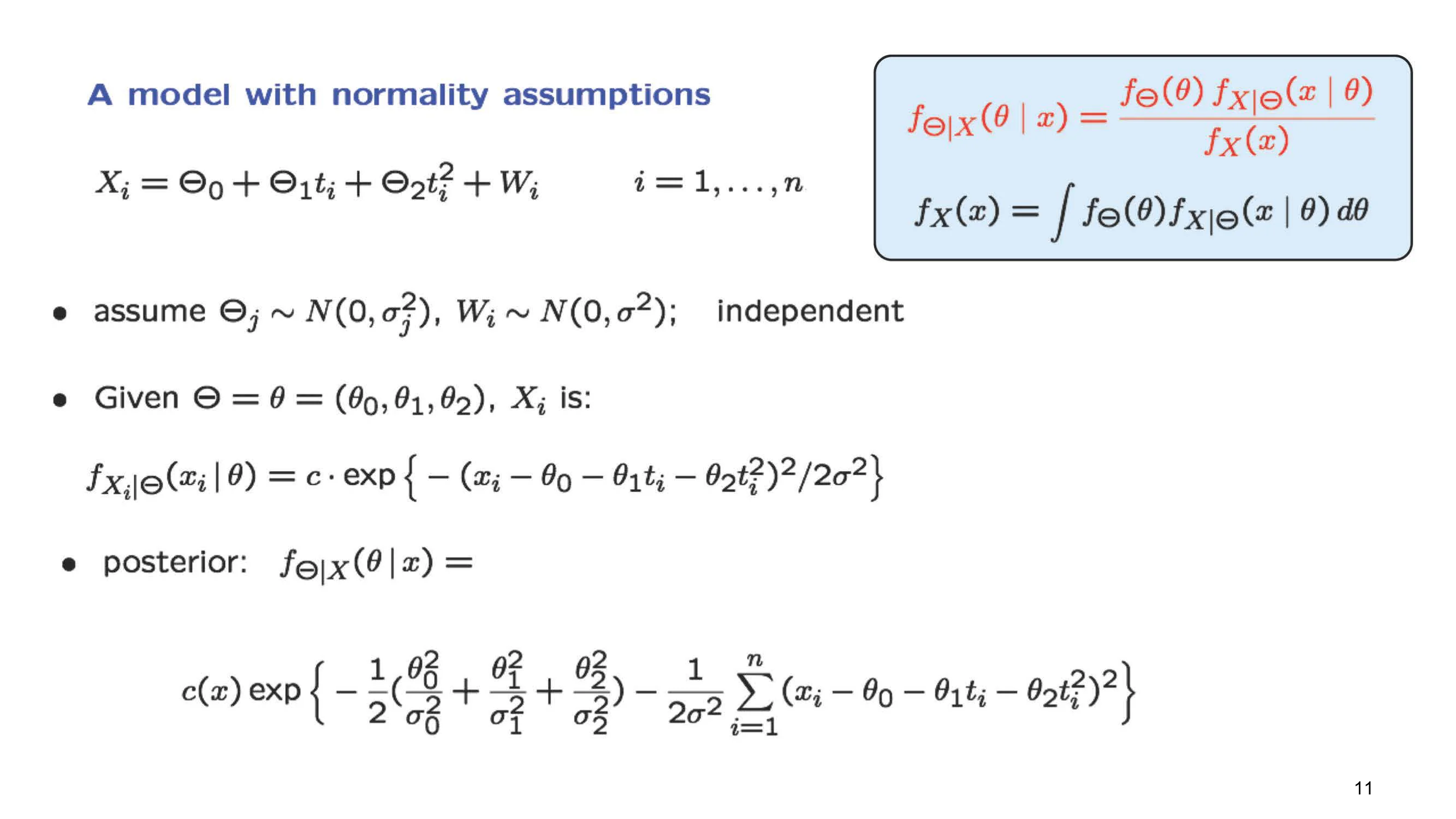
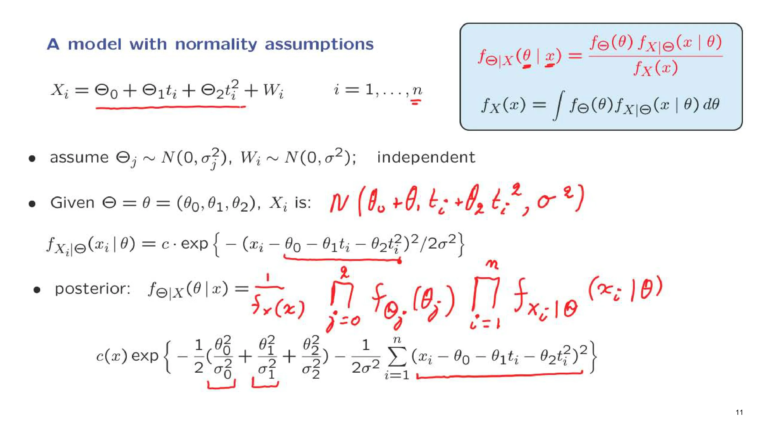
We would like to estimate the theta parameters on the basis of the observations. We will use, as usual, the appropriate form of Bayes' rule, which is this one, the Bayes' rule for continuous random variablescontinuous random variable / continuous random variables A continuous random variable is a random variable whose possible values form a continuum and are described by a density.. The only thing to notice is that in this notation here, X is an n-dimensional vector, because we have n observations. And theta, in this example, is a three-dimensional vector, because we have three unknown parameters. So wherever you see a theta or an X without a subscript, it should be interpreted as a vector.

Now, in order to calculate this posterior distribution, we need to put our hands on the conditional density of X. Actually, it is a joint density, because X is a vector, given the value of theta. The arguments are pretty much the same as in our previous examples, and they go as follows. Suppose that I tell you the value of the parameters, as here. Then we look at this equation. This quantity is now a constant. And we have a constant plus normal noise. So Xi is this normal noise whose mean is shifted by this constant. So Xi is going to be a normal random variable with a mean of theta 0 plus theta 1 ti plus theta 2 ti squared, and variance equal to the variance of Wi.

We know what the normal PDF is, so we can write it down. It is the usual exponential of a quadratic. And in this quadratic, we have Xi minus the mean of the normal random variable that we are dealing with.

Let us now continue and write down a formula for the posterior. We first have this denominator term, which does not involve any thetas and, as in previous examples, does not really concern us. Here we have the joint PDF of the vector of thetas. There are three of them. Because we assumed that the thetas are independent, the joint PDF factors as a product of individual PDFs. And then we have here the joint PDF of X conditioned on theta.

Now, with the same argument as in our previous discussion of the case of multiple observations, once I tell you the values of theta, then the Xi's are just functions of the noises. The noises are independent, so the Xi's are also independent. So in the conditional universe, where the value of theta is known, the Xi's are independent. And therefore, the joint PDF of the Xi's is equal to the product of the marginal PDFs of each one of the Xi's. But this marginal PDF in the conditional universe of the Xi's is something that we have already calculated. And so we know what each one of these densities is.

We can write them down, and we obtain an expression of this form. We have a normalizing constantnormalizing constant A normalizing constant is a factor that scales a function so it becomes a valid probability density. in the beginning. We have here a term that comes from the prior for theta 0, a prior for theta 1. Here is a typical term that comes from the density of Xi, which is this term up here. So here is what we have so far.

Show notesHide notes

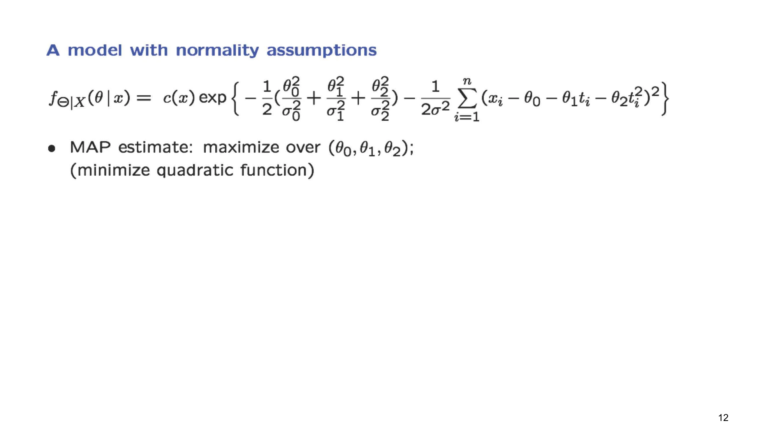
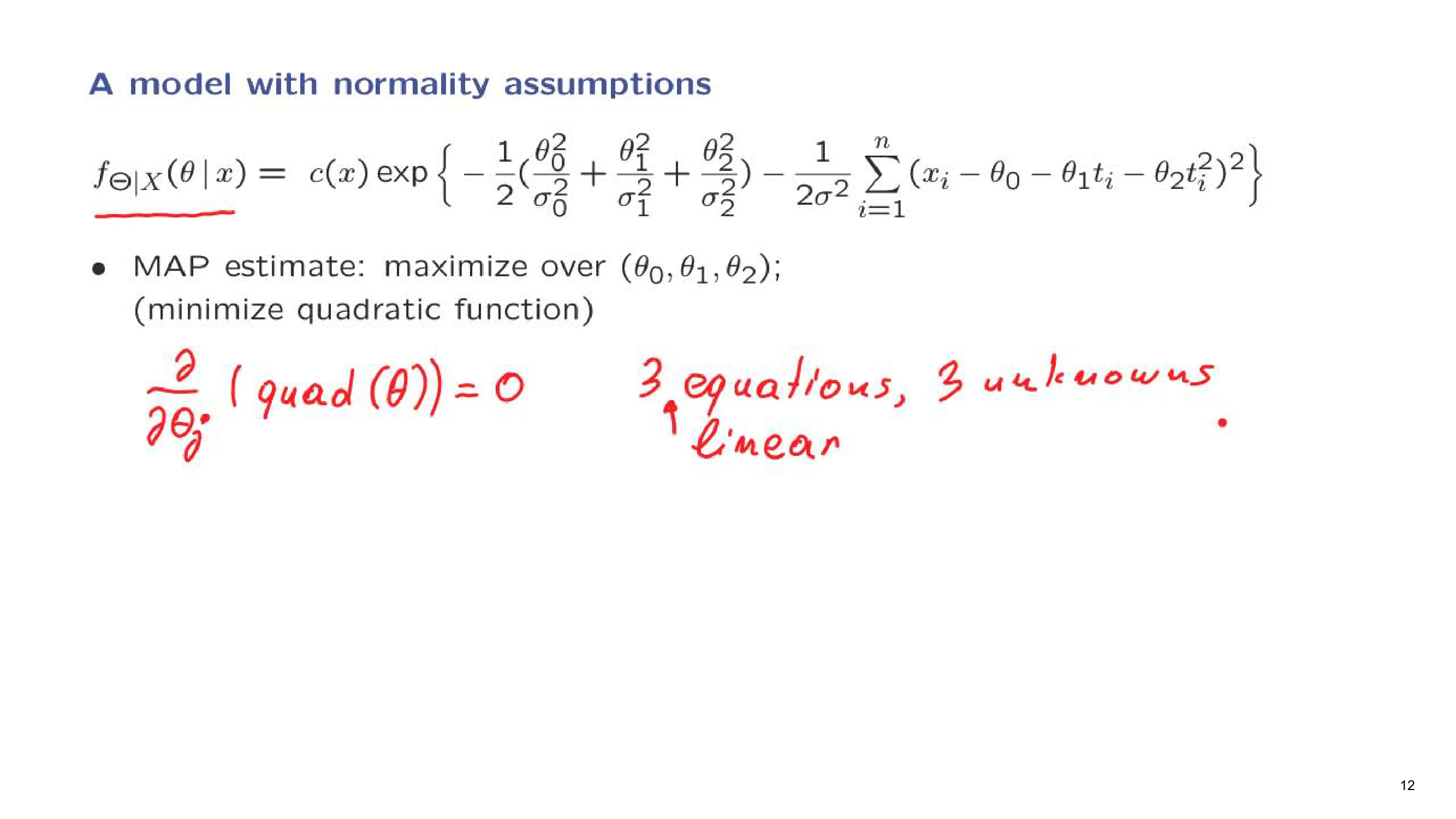
How should we now estimate theta if we wish to derive a point estimatepoint estimate A point estimate is a single value used to estimate an unknown parameter.? The natural process is to look for the maximum a posteriori probability estimate, which will maximize this expression over theta, find a set of theta parameters. It is a three-dimensional vector for which this quantity is largest. Equivalently, we can look at the exponent, get rid of the minus signs, and minimize the quadratic function that we obtain here.

How does one minimize a quadratic function? We take the derivatives with respect to each one of the parameters and set the derivative to 0. We will get, this way, three equations and three unknowns. And because it is a quadratic function of theta, these derivatives will be linear functions of theta. So these equations that we are dealing with will be linear equations. It is a system of three linear equations, which we can solve numerically. And this is what is usually done in practice. And this is exactly what it takes to calculate the maximum a posteriori probability estimate in this particular example that we have discussed. It turns out, as we will discuss later, that there are many interesting properties of this estimate which are quite general.

Linear regression preview

The trajectory estimation problem that we considered gives you a first glimpse into a large field that deals with linear normal modelslinear normal models Linear normal models are linear statistical models with normal assumptions for the relevant random variables.. In this segment, I will just give you a preview of what happens in that field, although we will not attempt to prove or justify anything. What happens in this field is that we're dealing with models where there are some underlying independent normal random variablesindependent normal random variables Independent normal random variables are Gaussian random variables that are independent of one another.. Then the random variables of interest, the unknown parameters, and the observations can all be expressed as linear functions of these independent normals. Since linear functions of independent normals are normal, this means in particular that the Theta_j and the X_i are all normal random variables.

Show notesHide notes

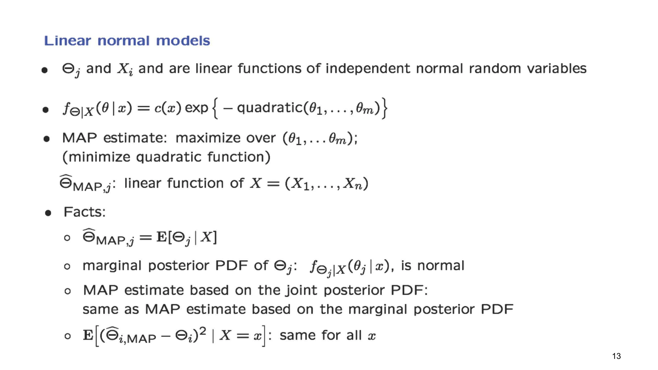
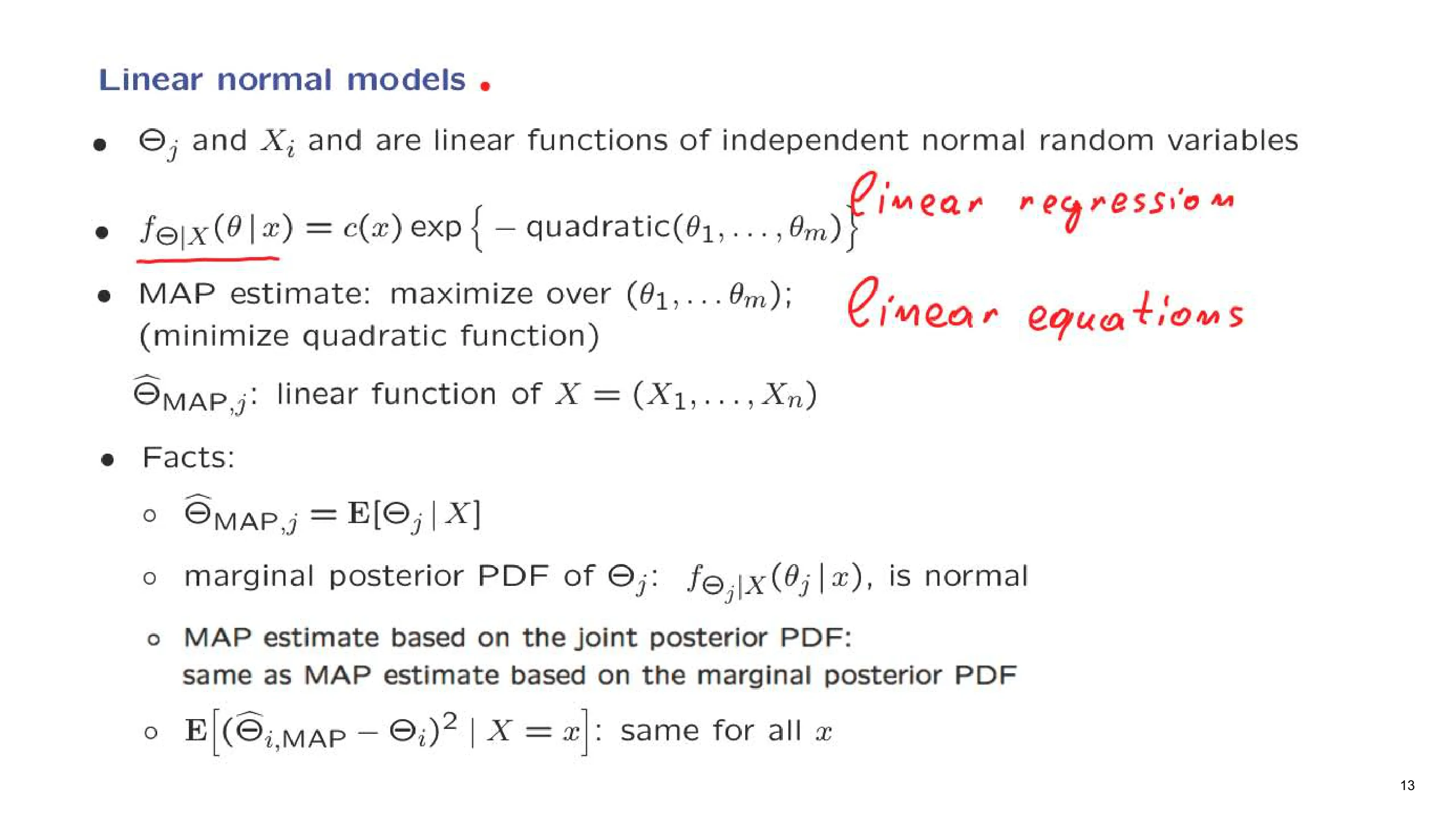
Carrying out inference within this class of models goes under the name of linear regressionlinear regression Linear regression is a linear model used to describe how a response variable depends on one or more predictors.. One can proceed using pretty much the same steps as we had in the trajectory estimation problem and write down formulas for the posterior. It turns out that in every case, the posterior of the parameter vector takes a form which is the exponential of the negative of a quadratic function of the parameters. This means, in particular, that in order to find the MAP estimate of the vector Theta, what we need to do is just minimize this quadratic function with respect to Theta. Minimizing a quadratic function is done by taking derivatives and setting them to 0, which leads us to a system of linear equations, exactly as in the trajectory inference problem.

This means that numerically, it is very simple to come up with a MAP estimate. There's an interesting fact that comes out of the algebra involved, namely that the MAP estimate of each one of the parameters turns out to also be a linear function of the observations. We saw this property in the estimators that we derived for simpler cases in this lecture sequence. It turns out that this property is still true. This is an appealing and desirable property, because it means that these estimators can be applied very efficiently in practice without having to do any complicated calculations.

Finally, there's a number of important facts, some of which we have seen in our examples, which are true in very big generality. One fact is that the maximum a posteriori probability estimate of some parameter turns out to be the same as the conditional expectation of that parameter. Furthermore, if you look at this joint density of all the Theta parameters, and from it you find the marginal density of the Theta parameters, always within this conditional universe, it turns out that this marginal posterior PDF is itself normal. Since it is normal, its mean, which is this quantity, is going to be equal to its peak. Therefore, it is also equal to the MAP estimate that would be derived from this marginal PDF.

So what do we have here? There are two ways of coming up with MAP estimates. One way is to find the peak of the joint PDF and then read out the different components of Theta. Another way of coming up with MAP estimates is to find, for each parameter, the marginal PDF and look at the peak of this marginal PDF. It turns out that for this model, these two approaches are going to give you the same answer. Whether you work with a marginal or with a joint, you get the same MAP estimates. This is a reassuring property to have.

Finally, as in the examples that we have worked in more detail, it turns out that the mean squared error conditioned on a particular observation is the same, no matter what the value of that observation was. Furthermore, there are fairly few simple and easily computable formulas that one can apply in order to find what this mean squared error is. So to summarize, this class of models that involve linear relations and normal random variables has a rich set of important and elegant properties. This is one of the reasons why these models are used so much in practice, and they're probably the most widely used class of statistical models.

Trajectory example and intervals

Let us now come back to the trajectory estimation problem that we introduced earlier. We have an object that moves vertically. At any given time t, the height at which the object is found is equal to this expression. It corresponds to the following: the object starts at time 0, at some initial height theta 0. It has an initial velocity of theta 1, but also has a certain acceleration. And if theta 2 is negative, this will be a downward acceleration, which means that the object eventually will turn and start going down.

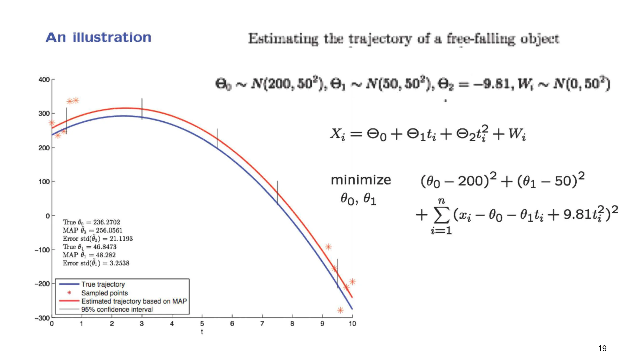
So this is a typical trajectory of such an object, where here we're plotting the height as a function of time. However, the thetas are unknown and they are random. We do not know what they are. So this blue curve is just a simulation where we drew values for those random variables at random. But if we were to simulate again, we might obtain a somewhat different blue curve, because the values of the thetas might have been different.

We do not observe the true trajectory directly. What we do observe is certain data points. At certain times, t_i, we make a measurement of the height of the object, except that this measurement is corrupted by some additive noise. This is the model that we introduced earlier. And our assumptions were that all the random variables involved, the thetas and the w's, were normal with 0 mean and were also independent.

In that case, we saw that maximizing the posterior distribution of the thetas, after taking logarithms, amounted to minimizing this quadratic function of the thetas. So once we have some data available in our hands, we look at this expression as a function of the thetas and find the thetas that are as good as possible in terms of this criterion. And this is the MAP methodology for this particular example.

Now, for the purposes of this illustration, we will change our assumptions a little bit. They will be as follows. Regarding the acceleration, we will take it to be a constant. The acceleration term often has to do with gravitational effects, which are known. So we will treat theta 2 as a constant. And that means that there is no point in having a prior distribution for theta 2. So this term here, which originated from the prior distribution of theta 2, is going to disappear.

We will take the variances of these basic random variables to be the same. And because of this, these constants here will all be the same. Therefore, we can take them outside this expression and outside the minimization. They will not matter. So we can remove them from the picture. The factor of 1/2 can also be removed similarly. It does not affect the minimization.

Finally, just in order to get a nicer illustration, instead of taking 0 means, we're assuming that the initial position has a mean of 200. So we're starting somewhere around here. And furthermore, the initial velocity has a mean of 50. So we expect the object to start moving upwards. How does this change the formulation? Well, remember that this term and this term originated from the priors for theta 0 and theta 1. If we now change the means, the priors will change. And what happens, if you recall the formula for the normal PDF and how the mean enters? After you take logarithms, you see that instead of having here theta 0, you should have theta 0 minus the mean of theta 0, squared. And this leads us to the following formulation.

So this is the formulation that we will consider. We obtain these data points. And for these particular data points, and for known times at which the measurements were taken, we put these numbers into this minimization, carried it out numerically. And this is what we got. We got estimates for the different parameters. And using these estimates, we can use this expression to construct an estimated trajectory. And the estimated trajectory is given by the red curve. It seems to be doing a somewhat reasonable job, but not quite; the distance between these two curves is quite substantial.

How could we do a little better? Why is it that we're not doing very well? Let's think intuitively. One of the parameters we wish to estimate is theta 1. And theta 1 is a velocity. Now, all of our measurements are concentrated at pretty much the same time. But if you measure an object only at a certain time, it is very difficult to estimate its velocity. A much better idea would be to try to measure the position of the object at different times and use that information to estimate velocity.

So let us instead, instead of taking all the measurements around the initial time, have five measurements in the beginning and five measurements towards the end. The total number of measurements in this example is the same as in the previous example. Once more, we generate a simulated trajectory according to the probability distributions that we are assuming. Then we generate data according to this model, and we wish to estimate this trajectory. We take the data, plug them into this minimization, carry it out numerically, and this is what we obtain.

So we see that here, we are doing a lot better. The estimated trajectory is quite close to the unknown blue trajectory, even though the data seem to be scattered quite a bit. This is a very nice property. But is it just an accident of this numerical experiment? Or, to put it differently, once you get your estimated trajectory, yes, it is true that it is close to the blue trajectory, but you do not necessarily know that fact. It is one thing to have an estimate that is close to the true value, and it's a different thing to have an estimate that you know is close to the true value.

So how could we get some guarantees that, indeed, this is the case, that we have good estimates? Here is how it goes. As we discussed before, the posterior distribution of the thetas, given the data, is normal. And for similar reasons, the posterior distribution of this quantity, which is the true position, it's what we denoted by X of tX of t X of t is the true position of the object at time t., is also normal. And in fact, what we obtain from this diagram is, at any given point, the maximum a posteriori probability estimate of the position X of t at that time.

However, besides just this point estimate, we have additional information. We know that the posterior distribution of X of tX of t X of t is the true position of the object at time t. is normal. And so, for example, at this time, this is the peak of the posterior. This is the maximum a posteriori probability estimate. But we are also able to calculate the variance of this posterior distribution. This is a calculation that's a bit complicated for the multivariate case, for the case where you have multiple unknown parameters. We will not get into it. But we did see earlier an example where we had a single unknown parameter, and in which we were able to calculate the variance of the posterior distribution. So the idea is somewhat similar.

So not only do we have an estimate for the position of the object at this particular time, but we also have a probability distribution for what the true position might be. And once we have such a posterior probability distribution, we can find an intervalconfidence interval / confidence intervals A confidence interval is an interval estimate for an unknown parameter, paired with a specified coverage level. with the property that 95% of the probability is inside that interval. In other words, we construct an interval with the property that the probability that X of t belongs to the interval, given the data, is, let's say, 0.95. Such an interval gives us useful information. Besides a point estimate, it also gives us a range of possible values. And outside this range, it is quite unlikely for the true trajectory to be out there.

So here we're showing some confidence intervalsconfidence interval / confidence intervals A confidence interval is an interval estimate for an unknown parameter, paired with a specified coverage level. that apply to different times. And they're pretty narrow. They're pretty small. And they indicate, they give us confidence, that we have pretty accurate estimates of the true trajectory.

These kinds of confidence intervals that we have discussed in the context of this example are called Bayesian confidence intervals. They are very useful when you report your results, to not just give point estimates, but also to provide confidence intervals.

Coming back to the bigger picture, what happened in this particular example is quite indicative of many real-world applications. One starts with a linear modellinear model A linear model expresses an outcome as a linear combination of predictors and unknown parameters, usually with random error. in which we have a linear relation between the variables that are unknown and the observations, but where the observations are also corrupted by noise. One makes certain normality and independence assumptions. And as long as the modeling has been done carefully and the assumptions are justified, then by carrying out this procedure, one usually obtains estimates that are very helpful and very informative.